import pandas as pd
import datetime as dt
import numpy as np
import matplotlib.pyplot as plt
import pandas_datareader as pdr
import scipy as sp
import seaborn as sns
import statsmodels.api as sm
import yfinance as yf
from statsmodels.graphics import tsaplots

import warnings

warnings.simplefilter("ignore")
plt.style.use("ggplot")
def filter_dunder(any_obj):
temp_list = dir(any_obj)
date_obj_meth_attr = []
for i in temp_list:
if i[0:2] != "__":
date_obj_meth_attr.append(i)
date_obj_meth_attr = {"meth_attr": date_obj_meth_attr}
return pd.DataFrame(date_obj_meth_attr)As a reminder, if you want to find data online to explore, check here: https://github.com/public-apis/public-apis
In this tutorial, we practice Pandas data manipulation techniques, which are extremely useful for practical time series analysis.
Import Data From Excel With Loop
The imported file here is a summary of three stock exchanges in US, i.e. NYSE, NASDAQ, AMEX, each stock exchange takes one sheet in the spreadsheet file.
We are going to import three sheets together by a loop.
First, instantiate an object for the Excel file, extract the sheet names.
listings = pd.read_csv("../dataset/nasdaq_listings.csv")
listings.head()| Stock Symbol | Company Name | Last Sale | Market Capitalization | IPO Year | Sector | Industry | Last Update | |
|---|---|---|---|---|---|---|---|---|
| 0 | AAPL | Apple Inc. | 141.05 | 7.400000e+11 | 1980 | Technology | Computer Manufacturing | 4/26/17 |
| 1 | GOOGL | Alphabet Inc. | 840.18 | 5.810000e+11 | NAN | Technology | Computer Software: Programming, Data Processing | 4/24/17 |
| 2 | GOOG | Alphabet Inc. | 823.56 | 5.690000e+11 | 2004 | Technology | Computer Software: Programming, Data Processing | 4/23/17 |
| 3 | MSFT | Microsoft Corporation | 64.95 | 5.020000e+11 | 1986 | Technology | Computer Software: Prepackaged Software | 4/26/17 |
| 4 | AMZN | Amazon.com, Inc. | 884.67 | 4.220000e+11 | 1997 | Consumer Services | Catalog/Specialty Distribution | 4/24/17 |
Pick The Largest Company in the Finance Sector
Let’s use the tickers as the index column.
listings = listings.set_index("Stock Symbol")
listings.head(5)| Company Name | Last Sale | Market Capitalization | IPO Year | Sector | Industry | Last Update | |
|---|---|---|---|---|---|---|---|
| Stock Symbol | |||||||
| AAPL | Apple Inc. | 141.05 | 7.400000e+11 | 1980 | Technology | Computer Manufacturing | 4/26/17 |
| GOOGL | Alphabet Inc. | 840.18 | 5.810000e+11 | NAN | Technology | Computer Software: Programming, Data Processing | 4/24/17 |
| GOOG | Alphabet Inc. | 823.56 | 5.690000e+11 | 2004 | Technology | Computer Software: Programming, Data Processing | 4/23/17 |
| MSFT | Microsoft Corporation | 64.95 | 5.020000e+11 | 1986 | Technology | Computer Software: Prepackaged Software | 4/26/17 |
| AMZN | Amazon.com, Inc. | 884.67 | 4.220000e+11 | 1997 | Consumer Services | Catalog/Specialty Distribution | 4/24/17 |
We can pick the tickers of top \(n\) financial companies.
This line of code is to extract the index number of top \(10\) financial companies.
n_largest = 10
tickers_large_financial = (
    listings.loc[listings["Sector"] == "Finance"]["Market Capitalization"]
    .nlargest(n_largest)
    .index.values
)
Then extract the ticker names.
Retrieve data from Yahoo finance.
start = dt.date(2010, 1, 1)
stocks_large_financial = yf.download(tickers=list(tickers_large_financial), start=start)
[ 0% ][********** 20% ] 2 of 10 completed[************** 30% ] 3 of 10 completed[******************* 40% ] 4 of 10 completed[**********************50% ] 5 of 10 completed[**********************60%**** ] 6 of 10 completed[**********************70%********* ] 7 of 10 completed[**********************80%************* ] 8 of 10 completed[**********************90%****************** ] 9 of 10 completed[*********************100%***********************] 10 of 10 completed
2 Failed downloads:
['WLTW', 'HBANO']: YFTzMissingError('$%ticker%: possibly delisted; no timezone found')stocks_large_financial["Close"].plot(subplots=True, layout=(5, 2), figsize=(16, 32))
plt.show()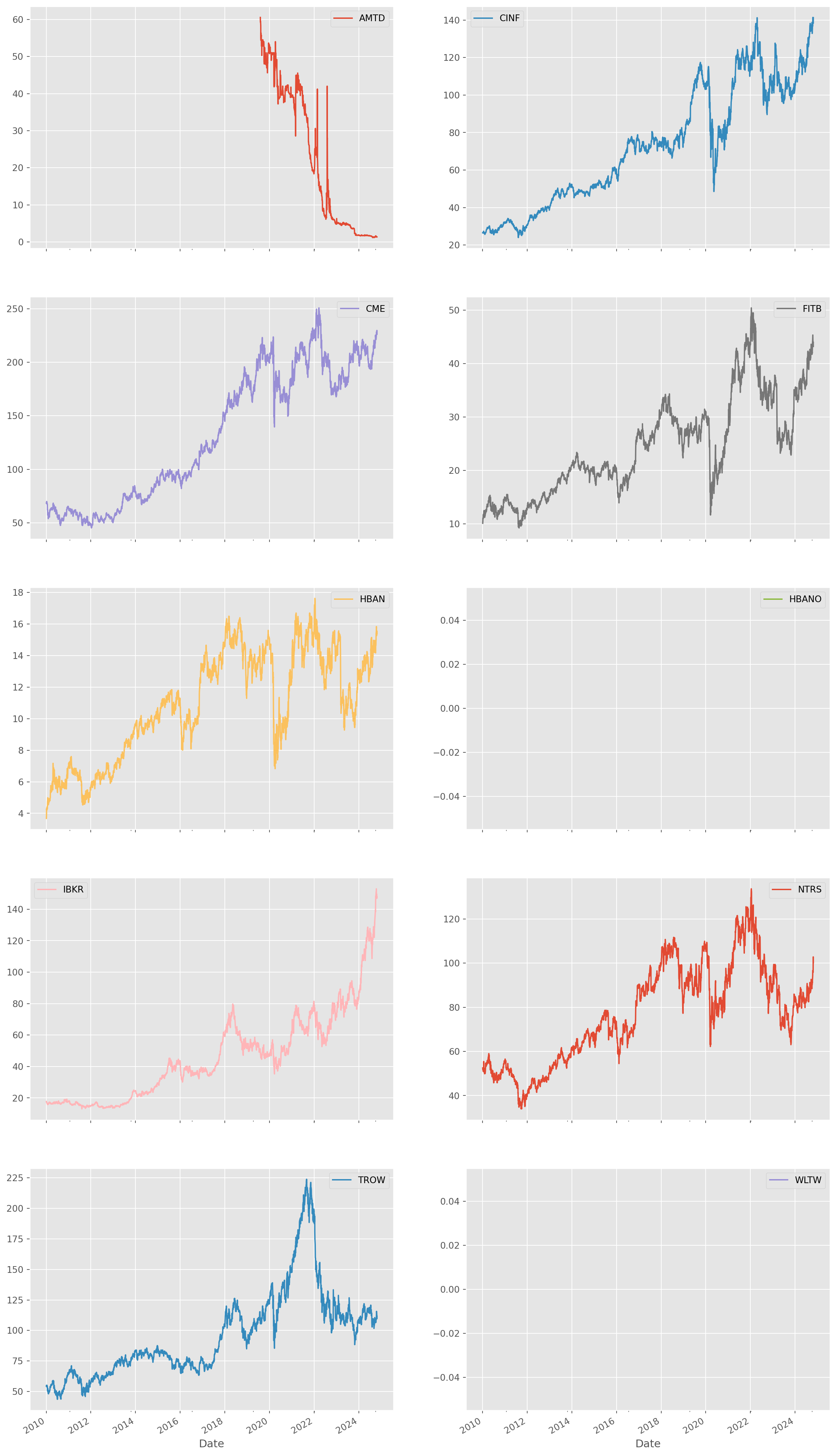
If some plot not shown, it could be that Yahoo changed the ticker name.
Pick The Large Major Pharmaceuticals In Health Care Sector
Let’s try again, pick the top pharmaceutical companies ranking from \(5\) to \(15\).
listings_health = listings[listings["Sector"] == "Health Care"]Take a look at what industries there are in Health Care.
hc_type = listings_health["Industry"].unique()
hc_type  # the type of health care companies
array(['Biotechnology: Biological Products (No Diagnostic Substances)',
'Major Pharmaceuticals', 'Medical/Nursing Services',
'Biotechnology: Commercial Physical & Biological Resarch',
'Industrial Specialties', 'Medical/Dental Instruments',
'Biotechnology: In Vitro & In Vivo Diagnostic Substances',
'Medical Specialities', 'Medical Electronics',
'Biotechnology: Electromedical & Electrotherapeutic Apparatus',
'Hospital/Nursing Management', 'Precision Instruments'],
dtype=object)Use Major Pharmaceuticals.
major_pharma_ranked = listings_health[
    listings_health["Industry"] == "Major Pharmaceuticals"
]["Market Capitalization"].sort_values(ascending=False)
major_pharma_picked_tickers = major_pharma_ranked[4:14].index
Again retrieve from Yahoo finance.
stocks_pharma_picked = yf.download(list(major_pharma_picked_tickers), start)[ 0% ][********** 20% ] 2 of 10 completed[************** 30% ] 3 of 10 completed[******************* 40% ] 4 of 10 completed[**********************50% ] 5 of 10 completed[**********************60%**** ] 6 of 10 completed[**********************70%********* ] 7 of 10 completed[**********************80%************* ] 8 of 10 completed[**********************80%************* ] 8 of 10 completed[*********************100%***********************] 10 of 10 completed
1 Failed download:
['MYL']: YFTzMissingError('$%ticker%: possibly delisted; no timezone found')Use only close price.
stocks_pharma_picked_close = stocks_pharma_picked["Close"]stocks_pharma_picked_close.plot(subplots=True, layout=(5, 2), figsize=(16, 32))
plt.show()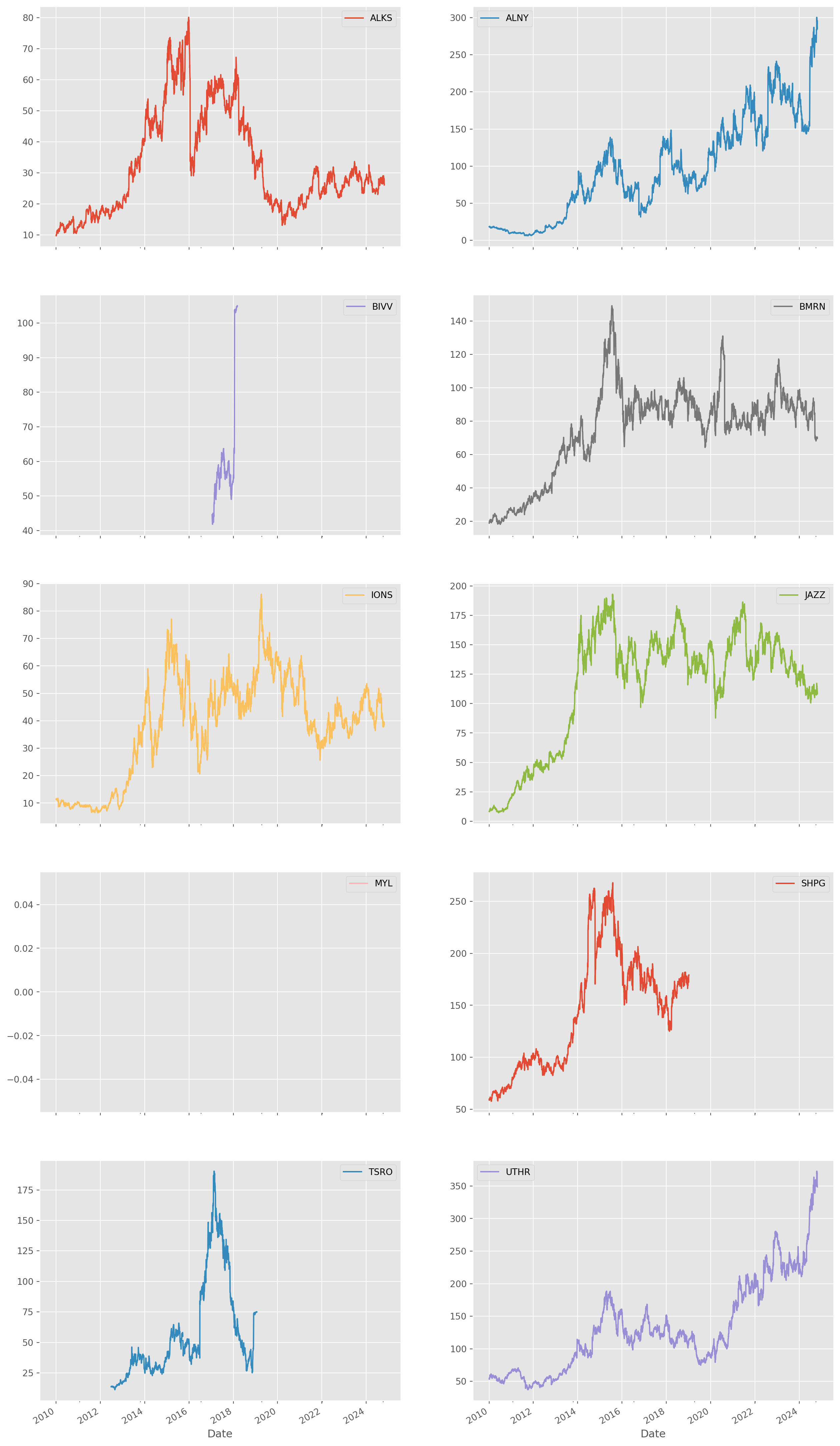
Multiple Criteria in .loc
Multiple selection criteria are joined by & sign.
listings_filtered = listings[listings["IPO Year"] != "NAN"]
listings_filtered = listings_filtered.loc[
    listings_filtered["IPO Year"].astype(int) > 2008
]
Density Plot of Daily Returns
Use the pharmaceutical data we extracted to draw distributions of daily return.
pharma_growth = stocks_pharma_picked_close.pct_change()
plt.figure(figsize=(8, 5))
for column in pharma_growth.columns:
    sns.histplot(pharma_growth[column], label=column)
plt.legend()
plt.show()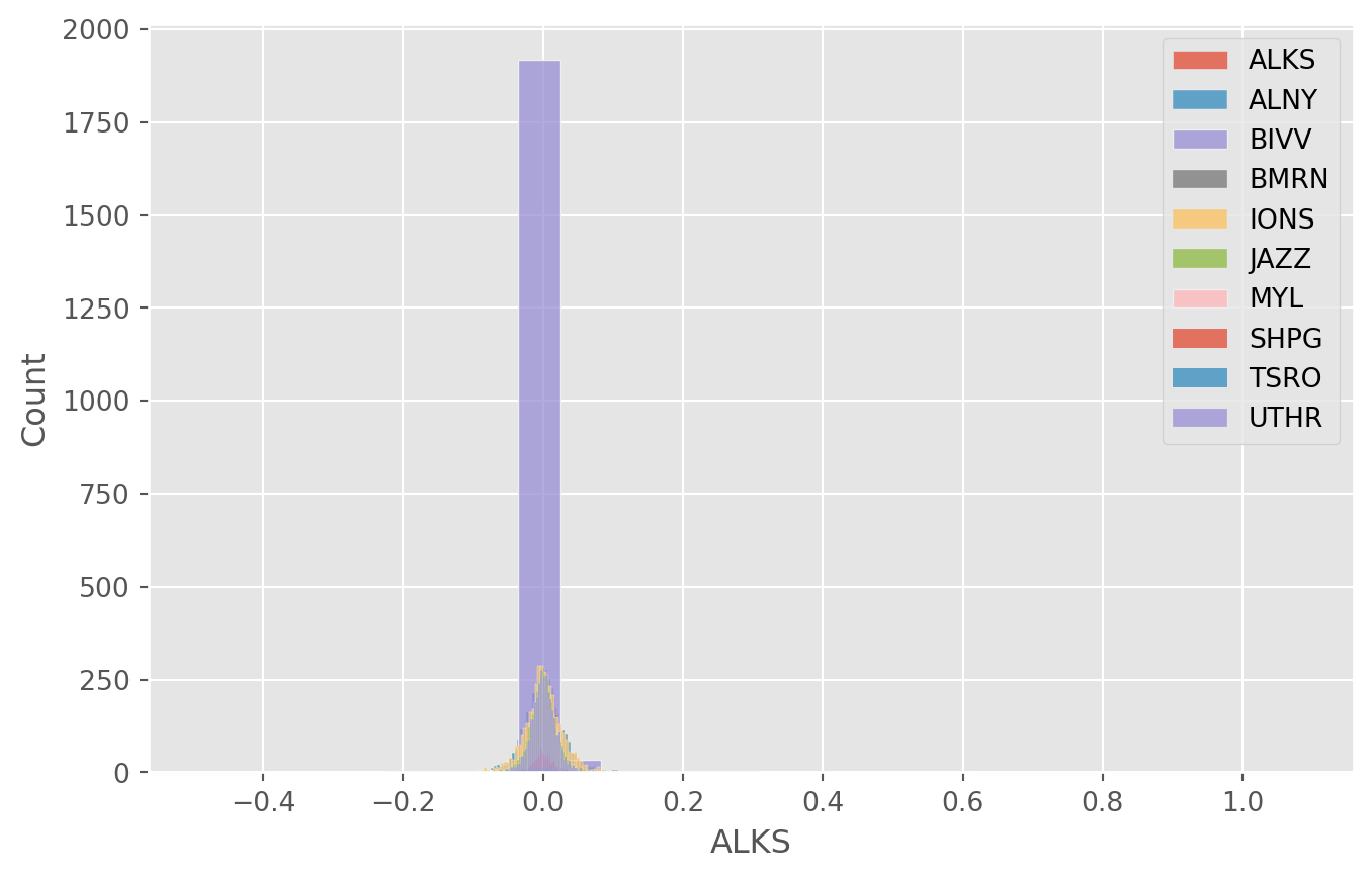
Count Sectors
Count how many companies in each sector.
listings["Sector"].value_counts().sort_values(ascending=True).plot(kind="barh")
plt.show()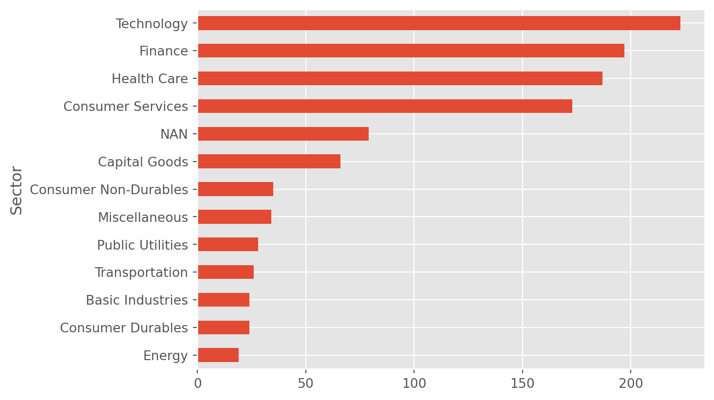
You can count companies in industries too.
listings["Industry"].value_counts().sort_values(ascending=True).plot(
    kind="barh", figsize=(8, 40)
)
plt.show()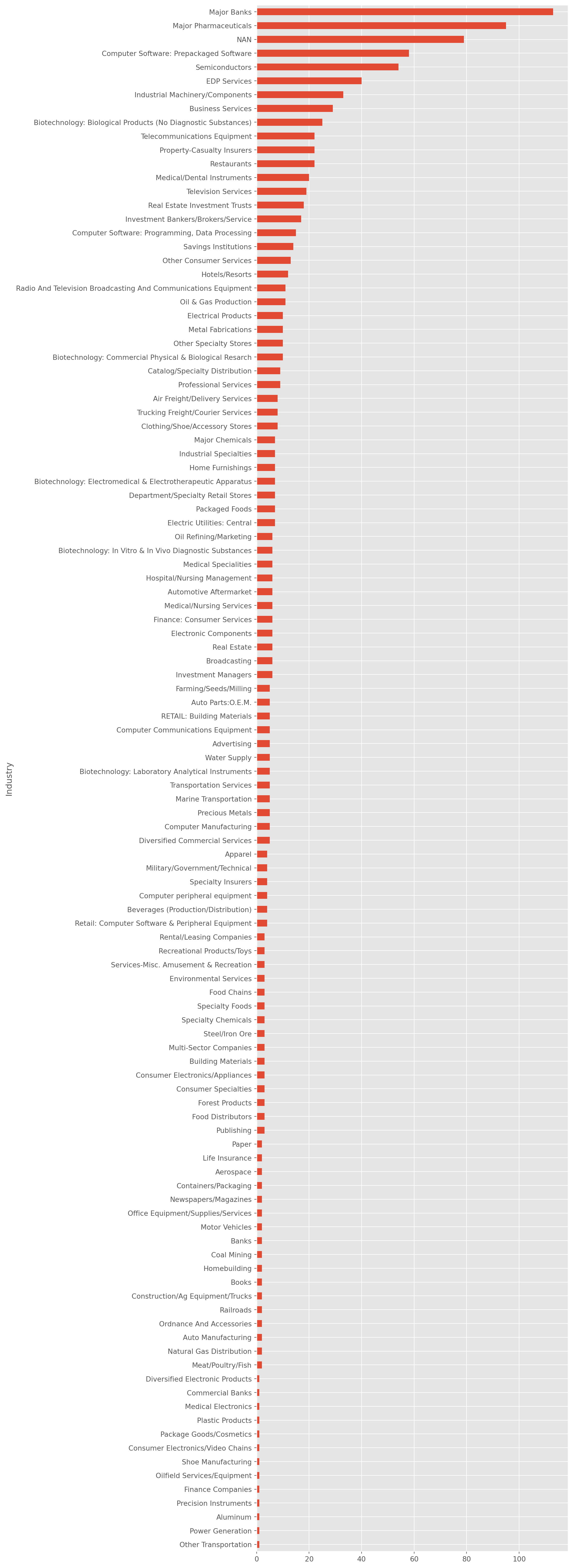
Group By Multiple Criteria Then Unstack
First we group the data by sector and exchange, then take mean of all numerical values. Of course it would be ridiculous to calculate the means of IPO year.
listings.head()| Company Name | Last Sale | Market Capitalization | IPO Year | Sector | Industry | Last Update | |
|---|---|---|---|---|---|---|---|
| Stock Symbol | |||||||
| AAPL | Apple Inc. | 141.05 | 7.400000e+11 | 1980 | Technology | Computer Manufacturing | 4/26/17 |
| GOOGL | Alphabet Inc. | 840.18 | 5.810000e+11 | NAN | Technology | Computer Software: Programming, Data Processing | 4/24/17 |
| GOOG | Alphabet Inc. | 823.56 | 5.690000e+11 | 2004 | Technology | Computer Software: Programming, Data Processing | 4/23/17 |
| MSFT | Microsoft Corporation | 64.95 | 5.020000e+11 | 1986 | Technology | Computer Software: Prepackaged Software | 4/26/17 |
| AMZN | Amazon.com, Inc. | 884.67 | 4.220000e+11 | 1997 | Consumer Services | Catalog/Specialty Distribution | 4/24/17 |
group_mean = listings.groupby(["Sector", "Industry"]).mean(numeric_only=True)
group_mean.head(21)| Last Sale | Market Capitalization | ||
|---|---|---|---|
| Sector | Industry | ||
| Basic Industries | Aluminum | 11.640000 | 1.015670e+09 |
| Environmental Services | 81.920000 | 6.983447e+09 | |
| Forest Products | 80.413333 | 1.419229e+09 | |
| Home Furnishings | 34.950000 | 5.538917e+08 | |
| Homebuilding | 114.800000 | 1.032427e+09 | |
| Major Chemicals | 51.012857 | 1.690641e+09 | |
| Paper | 11.450000 | 7.439483e+08 | |
| Precious Metals | 40.369000 | 2.649588e+09 | |
| Steel/Iron Ore | 32.910000 | 7.976835e+09 | |
| Water Supply | 28.373333 | 8.600694e+08 | |
| Capital Goods | Aerospace | 35.965000 | 1.490300e+09 |
| Auto Manufacturing | 184.315000 | 3.615822e+10 | |
| Auto Parts:O.E.M. | 46.092000 | 3.720569e+09 | |
| Biotechnology: Laboratory Analytical Instruments | 90.512000 | 7.584176e+09 | |
| Building Materials | 38.593333 | 1.120403e+09 | |
| Construction/Ag Equipment/Trucks | 42.335000 | 9.691799e+08 | |
| Electrical Products | 53.844000 | 2.089606e+09 | |
| Electronic Components | 63.415000 | 8.455846e+09 | |
| Homebuilding | 30.070000 | 6.492711e+08 | |
| Industrial Machinery/Components | 43.774737 | 2.769587e+09 | |
| Industrial Specialties | 12.565000 | 7.284660e+08 |
Unstack method is able to flatten the dataset by aligning the second indices, here is Exchange.
gm_unstacked = group_mean.unstack()
gm_unstacked| Last Sale | ... | Market Capitalization | |||||||||||||||||||
|---|---|---|---|---|---|---|---|---|---|---|---|---|---|---|---|---|---|---|---|---|---|
| Industry | Advertising | Aerospace | Air Freight/Delivery Services | Aluminum | Apparel | Auto Manufacturing | Auto Parts:O.E.M. | Automotive Aftermarket | Banks | Beverages (Production/Distribution) | ... | Shoe Manufacturing | Specialty Chemicals | Specialty Foods | Specialty Insurers | Steel/Iron Ore | Telecommunications Equipment | Television Services | Transportation Services | Trucking Freight/Courier Services | Water Supply |
| Sector | |||||||||||||||||||||
| Basic Industries | NaN | NaN | NaN | 11.64 | NaN | NaN | NaN | NaN | NaN | NaN | ... | NaN | NaN | NaN | NaN | 7.976835e+09 | NaN | NaN | NaN | NaN | 8.600694e+08 |
| Capital Goods | NaN | 35.965 | NaN | NaN | NaN | 184.315 | 46.092 | NaN | NaN | NaN | ... | NaN | 1.019154e+09 | NaN | NaN | 9.171397e+08 | NaN | NaN | NaN | NaN | NaN |
| Consumer Durables | NaN | NaN | NaN | NaN | NaN | NaN | NaN | 47.916 | NaN | NaN | ... | NaN | 8.351350e+08 | NaN | NaN | NaN | 1.830985e+09 | NaN | NaN | NaN | NaN |
| Consumer Non-Durables | NaN | NaN | NaN | NaN | 63.8225 | NaN | NaN | NaN | NaN | 96.155 | ... | 2.184033e+09 | NaN | 2.379612e+09 | NaN | NaN | NaN | NaN | NaN | NaN | NaN |
| Consumer Services | 11.820000 | NaN | NaN | NaN | NaN | NaN | NaN | 52.450 | NaN | NaN | ... | NaN | NaN | NaN | NaN | NaN | 1.057490e+09 | 3.209950e+10 | 7.247331e+09 | NaN | NaN |
| Energy | NaN | NaN | NaN | NaN | NaN | NaN | NaN | NaN | NaN | NaN | ... | NaN | NaN | NaN | NaN | NaN | NaN | NaN | NaN | NaN | NaN |
| Finance | NaN | NaN | NaN | NaN | NaN | NaN | NaN | NaN | 20.0 | NaN | ... | NaN | NaN | NaN | 6.539013e+09 | NaN | NaN | NaN | NaN | NaN | NaN |
| Health Care | NaN | NaN | NaN | NaN | NaN | NaN | NaN | NaN | NaN | NaN | ... | NaN | NaN | NaN | NaN | NaN | NaN | NaN | NaN | NaN | NaN |
| Miscellaneous | NaN | NaN | NaN | NaN | NaN | NaN | NaN | NaN | NaN | NaN | ... | NaN | NaN | NaN | NaN | NaN | NaN | NaN | NaN | NaN | NaN |
| NAN | NaN | NaN | NaN | NaN | NaN | NaN | NaN | NaN | NaN | NaN | ... | NaN | NaN | NaN | NaN | NaN | NaN | NaN | NaN | NaN | NaN |
| Public Utilities | NaN | NaN | NaN | NaN | NaN | NaN | NaN | NaN | NaN | NaN | ... | NaN | NaN | NaN | NaN | NaN | 9.041919e+09 | NaN | NaN | NaN | 5.955152e+08 |
| Technology | 53.806667 | NaN | NaN | NaN | NaN | NaN | NaN | NaN | NaN | NaN | ... | NaN | NaN | NaN | NaN | NaN | 3.929865e+09 | NaN | NaN | NaN | NaN |
| Transportation | NaN | NaN | 56.66625 | NaN | NaN | NaN | NaN | NaN | NaN | NaN | ... | NaN | NaN | NaN | NaN | NaN | NaN | NaN | 1.461312e+09 | 3.225595e+09 | NaN |
13 rows × 224 columns
Aggregate Functions
Aggregate function is not particular useful, but still here we present its common use for statistical summary presentation.
listings.groupby(["Sector", "Industry"])["Market Capitalization"].agg(
    Mean="mean", Median="median", STD="std"
).unstack()| Mean | ... | STD | |||||||||||||||||||
|---|---|---|---|---|---|---|---|---|---|---|---|---|---|---|---|---|---|---|---|---|---|
| Industry | Advertising | Aerospace | Air Freight/Delivery Services | Aluminum | Apparel | Auto Manufacturing | Auto Parts:O.E.M. | Automotive Aftermarket | Banks | Beverages (Production/Distribution) | ... | Shoe Manufacturing | Specialty Chemicals | Specialty Foods | Specialty Insurers | Steel/Iron Ore | Telecommunications Equipment | Television Services | Transportation Services | Trucking Freight/Courier Services | Water Supply |
| Sector | |||||||||||||||||||||
| Basic Industries | NaN | NaN | NaN | 1.015670e+09 | NaN | NaN | NaN | NaN | NaN | NaN | ... | NaN | NaN | NaN | NaN | NaN | NaN | NaN | NaN | NaN | 2.800612e+08 |
| Capital Goods | NaN | 1.490300e+09 | NaN | NaN | NaN | 3.615822e+10 | 3.720569e+09 | NaN | NaN | NaN | ... | NaN | NaN | NaN | NaN | 3.688554e+08 | NaN | NaN | NaN | NaN | NaN |
| Consumer Durables | NaN | NaN | NaN | NaN | NaN | NaN | NaN | 5.828704e+09 | NaN | NaN | ... | NaN | 6.482536e+07 | NaN | NaN | NaN | 1.212232e+09 | NaN | NaN | NaN | NaN |
| Consumer Non-Durables | NaN | NaN | NaN | NaN | 6.263316e+09 | NaN | NaN | NaN | NaN | 8.045628e+09 | ... | NaN | NaN | 1.526457e+09 | NaN | NaN | NaN | NaN | NaN | NaN | NaN |
| Consumer Services | 6.589818e+08 | NaN | NaN | NaN | NaN | NaN | NaN | 1.708098e+09 | NaN | NaN | ... | NaN | NaN | NaN | NaN | NaN | 6.369712e+08 | 4.168866e+10 | 1.036975e+10 | NaN | NaN |
| Energy | NaN | NaN | NaN | NaN | NaN | NaN | NaN | NaN | NaN | NaN | ... | NaN | NaN | NaN | NaN | NaN | NaN | NaN | NaN | NaN | NaN |
| Finance | NaN | NaN | NaN | NaN | NaN | NaN | NaN | NaN | 7.670564e+08 | NaN | ... | NaN | NaN | NaN | 7.459145e+09 | NaN | NaN | NaN | NaN | NaN | NaN |
| Health Care | NaN | NaN | NaN | NaN | NaN | NaN | NaN | NaN | NaN | NaN | ... | NaN | NaN | NaN | NaN | NaN | NaN | NaN | NaN | NaN | NaN |
| Miscellaneous | NaN | NaN | NaN | NaN | NaN | NaN | NaN | NaN | NaN | NaN | ... | NaN | NaN | NaN | NaN | NaN | NaN | NaN | NaN | NaN | NaN |
| NAN | NaN | NaN | NaN | NaN | NaN | NaN | NaN | NaN | NaN | NaN | ... | NaN | NaN | NaN | NaN | NaN | NaN | NaN | NaN | NaN | NaN |
| Public Utilities | NaN | NaN | NaN | NaN | NaN | NaN | NaN | NaN | NaN | NaN | ... | NaN | NaN | NaN | NaN | NaN | 1.705657e+10 | NaN | NaN | NaN | 1.151748e+07 |
| Technology | 2.218324e+09 | NaN | NaN | NaN | NaN | NaN | NaN | NaN | NaN | NaN | ... | NaN | NaN | NaN | NaN | NaN | NaN | NaN | NaN | NaN | NaN |
| Transportation | NaN | NaN | 6.136594e+09 | NaN | NaN | NaN | NaN | NaN | NaN | NaN | ... | NaN | NaN | NaN | NaN | NaN | NaN | NaN | 1.513037e+08 | 3.361975e+09 | NaN |
13 rows × 336 columns
Countplot
Let’s find all companies which are listed after year \(2000\).
listings_without_nans = listings[listings["IPO Year"] != "NAN"]
listings_post2000 = listings_without_nans[
    listings_without_nans["IPO Year"].astype(int) > 2000
]
listings_post2000.head()| Company Name | Last Sale | Market Capitalization | IPO Year | Sector | Industry | Last Update | |
|---|---|---|---|---|---|---|---|
| Stock Symbol | |||||||
| GOOG | Alphabet Inc. | 823.56 | 5.690000e+11 | 2004 | Technology | Computer Software: Programming, Data Processing | 4/23/17 |
| FB | Facebook, Inc. | 139.39 | 4.030000e+11 | 2012 | Technology | Computer Software: Programming, Data Processing | 4/26/17 |
| AVGO | Broadcom Limited | 211.32 | 8.481592e+10 | 2009 | Technology | Semiconductors | 4/26/17 |
| NFLX | Netflix, Inc. | 142.92 | 6.151442e+10 | 2002 | Consumer Services | Consumer Electronics/Video Chains | 4/24/17 |
| TSLA | Tesla, Inc. | 304.00 | 4.961483e+10 | 2010 | Capital Goods | Auto Manufacturing | 4/26/17 |
However you can see the year type is not integers, but rather floats. Use .astype to convert the data type.
listings_post2000["IPO Year"] = listings_post2000["IPO Year"].astype(int)
listings_post2000.head()| Company Name | Last Sale | Market Capitalization | IPO Year | Sector | Industry | Last Update | |
|---|---|---|---|---|---|---|---|
| Stock Symbol | |||||||
| GOOG | Alphabet Inc. | 823.56 | 5.690000e+11 | 2004 | Technology | Computer Software: Programming, Data Processing | 4/23/17 |
| FB | Facebook, Inc. | 139.39 | 4.030000e+11 | 2012 | Technology | Computer Software: Programming, Data Processing | 4/26/17 |
| AVGO | Broadcom Limited | 211.32 | 8.481592e+10 | 2009 | Technology | Semiconductors | 4/26/17 |
| NFLX | Netflix, Inc. | 142.92 | 6.151442e+10 | 2002 | Consumer Services | Consumer Electronics/Video Chains | 4/24/17 |
| TSLA | Tesla, Inc. | 304.00 | 4.961483e+10 | 2010 | Capital Goods | Auto Manufacturing | 4/26/17 |
Now we can plot the listings in each year after \(2000\) in every exchanges.
plt.figure(figsize=(12, 6))
sns.countplot(x="IPO Year", hue="Industry", data=listings_post2000)
plt.show()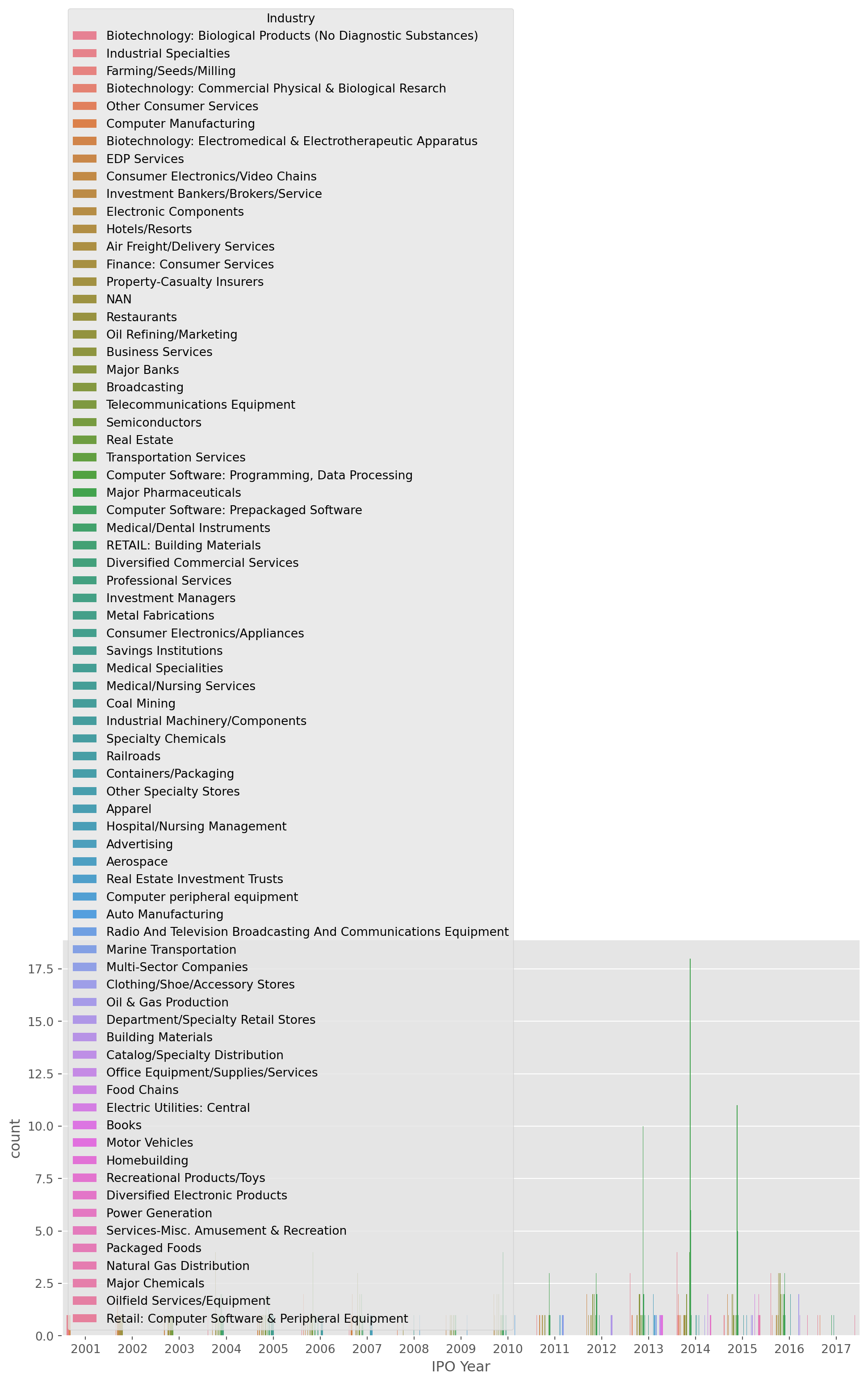
Merging Different Time Series
This example shows that bonds and stock markets are not open in the same days. Especially useful when you retrieve the data from different sources.
set is the function to return a set with unique values, the difference of both sets are the days that either of them is closed, but not both.
start = dt.datetime(2018, 1, 1)
sp500 = pdr.data.DataReader("sp500", "fred", start).dropna()
us10y = pdr.data.DataReader("DGS10", "fred", start).dropna()
A simple trick can show if a specific date presents in either series.
try:
    sp500.loc["2018-10-08"]
except:
print("No data on this date")try:
us10y.loc["2018-10-08"]
except:
print("No data on this date")No data on this dateThe set of S&P500 dates minus the set of US10y returns the dates that stocks opened while bonds closed, vice versa we obtain the dates bonds market opened.
set(sp500.index) - set(us10y.index) # A - B return a set of elements that only A has{Timestamp('2018-10-08 00:00:00'),
Timestamp('2018-11-12 00:00:00'),
Timestamp('2019-10-14 00:00:00'),
Timestamp('2019-11-11 00:00:00'),
Timestamp('2020-10-12 00:00:00'),
Timestamp('2020-11-11 00:00:00'),
Timestamp('2021-10-11 00:00:00'),
Timestamp('2021-11-11 00:00:00'),
Timestamp('2022-10-10 00:00:00'),
Timestamp('2022-11-11 00:00:00'),
Timestamp('2023-10-09 00:00:00'),
Timestamp('2024-10-14 00:00:00'),
Timestamp('2024-10-25 00:00:00')}set(us10y.index) - set(sp500.index) # B - A return a set of elements that only B has{Timestamp('2021-04-02 00:00:00'), Timestamp('2023-04-07 00:00:00')}inner means obtain the intersection set of two time indices, i.e. the days both markets open in this case.
us10y.join(sp500, how="inner")| DGS10 | sp500 | |
|---|---|---|
| DATE | ||
| 2018-01-02 | 2.46 | 2695.81 |
| 2018-01-03 | 2.44 | 2713.06 |
| 2018-01-04 | 2.46 | 2723.99 |
| 2018-01-05 | 2.47 | 2743.15 |
| 2018-01-08 | 2.49 | 2747.71 |
| ... | ... | ... |
| 2024-10-18 | 4.08 | 5864.67 |
| 2024-10-21 | 4.19 | 5853.98 |
| 2024-10-22 | 4.20 | 5851.20 |
| 2024-10-23 | 4.24 | 5797.42 |
| 2024-10-24 | 4.21 | 5809.86 |
1703 rows × 2 columns
However, pandas_reader has a simpler solution, by importing as a group from FRED, which solve this issue automatically.
code_name = ["sp500", "DGS10"]
start = dt.datetime(2018, 1, 1)
df = pdr.data.DataReader(code_name, "fred", start).dropna()
Check if both sets of indices are the same this time.
print(set(df["sp500"].index) - set(df["DGS10"].index))
print(set(df["DGS10"].index) - set(df["sp500"].index))
set()
set()The sets are empty, we have obtained the same time indices.
Period function
Any datetime object can display a timestamp.
time_stamp = pd.Timestamp(dt.datetime(2021, 12, 25))
time_stamp
Timestamp('2021-12-25 00:00:00')filter_dunder(time_stamp) # take a look what methods or features| meth_attr | |
|---|---|
| 0 | _creso |
| 1 | _date_repr |
| 2 | _from_dt64 |
| 3 | _from_value_and_reso |
| 4 | _repr_base |
| ... | ... |
| 78 | value |
| 79 | week |
| 80 | weekday |
| 81 | weekofyear |
| 82 | year |
83 rows × 1 columns
print(time_stamp.year)
print(time_stamp.month)
print(time_stamp.day)
print(time_stamp.day_name())
2021
12
25
Saturdayprint(time_stamp)2021-12-25 00:00:00The period function literally creates a period, it is not a single point of time anymore.
period = pd.Period("2021-8")
period
Period('2021-08', 'M')period_2 = pd.Period("2021-8-28", "D")
period_2Period('2021-08-28', 'D')print(period + 2)2021-10print(period_2 - 10)2021-08-18Sequence of Time
Each object of date_range is a Timestamp object.
index = pd.date_range(start="2010-12", end="2021-12", freq="M")
index
DatetimeIndex(['2010-12-31', '2011-01-31', '2011-02-28', '2011-03-31',
'2011-04-30', '2011-05-31', '2011-06-30', '2011-07-31',
'2011-08-31', '2011-09-30',
...
'2021-02-28', '2021-03-31', '2021-04-30', '2021-05-31',
'2021-06-30', '2021-07-31', '2021-08-31', '2021-09-30',
'2021-10-31', '2021-11-30'],
dtype='datetime64[ns]', length=132, freq='ME')Convert to period index. The difference is that period index is usually for flow variables, it shows the accumulation rather than a snap shot of status.
index.to_period()PeriodIndex(['2010-12', '2011-01', '2011-02', '2011-03', '2011-04', '2011-05',
'2011-06', '2011-07', '2011-08', '2011-09',
...
'2021-02', '2021-03', '2021-04', '2021-05', '2021-06', '2021-07',
'2021-08', '2021-09', '2021-10', '2021-11'],
dtype='period[M]', length=132)Let’s print \(10\) days from 1st Dec 2021 onward.
index_2 = pd.date_range(start="2021-12-1", periods=10)
for day in index_2:
    print(str(day.day) + ":" + day.day_name())
1:Wednesday
2:Thursday
3:Friday
4:Saturday
5:Sunday
6:Monday
7:Tuesday
8:Wednesday
9:Thursday
10:Fridayindex_2DatetimeIndex(['2021-12-01', '2021-12-02', '2021-12-03', '2021-12-04',
'2021-12-05', '2021-12-06', '2021-12-07', '2021-12-08',
'2021-12-09', '2021-12-10'],
dtype='datetime64[ns]', freq='D')Create a Time Series
To simulate time series, we need to generate time series with proper indices, something matching the real time series.
Let’s use the time index generated above, give it a name Time.
time_series = pd.DataFrame({"Time": index})time_series.info()<class 'pandas.core.frame.DataFrame'>
RangeIndex: 132 entries, 0 to 131
Data columns (total 1 columns):
# Column Non-Null Count Dtype
--- ------ -------------- -----
0 Time 132 non-null datetime64[ns]
dtypes: datetime64[ns](1)
memory usage: 1.2 KBdata = np.random.randn(len(index), 2) # two columns of Gaussian generated variablesTwo series and an index, a simple line of code to create.
time_series = pd.DataFrame(data=data, index=index, columns=["Series_1", "Series_2"])Pandas plot function is convenient for fast plotting, FYI colormap is here .
time_series.plot(colormap="Paired", figsize=(16, 8), subplots=True)
plt.show()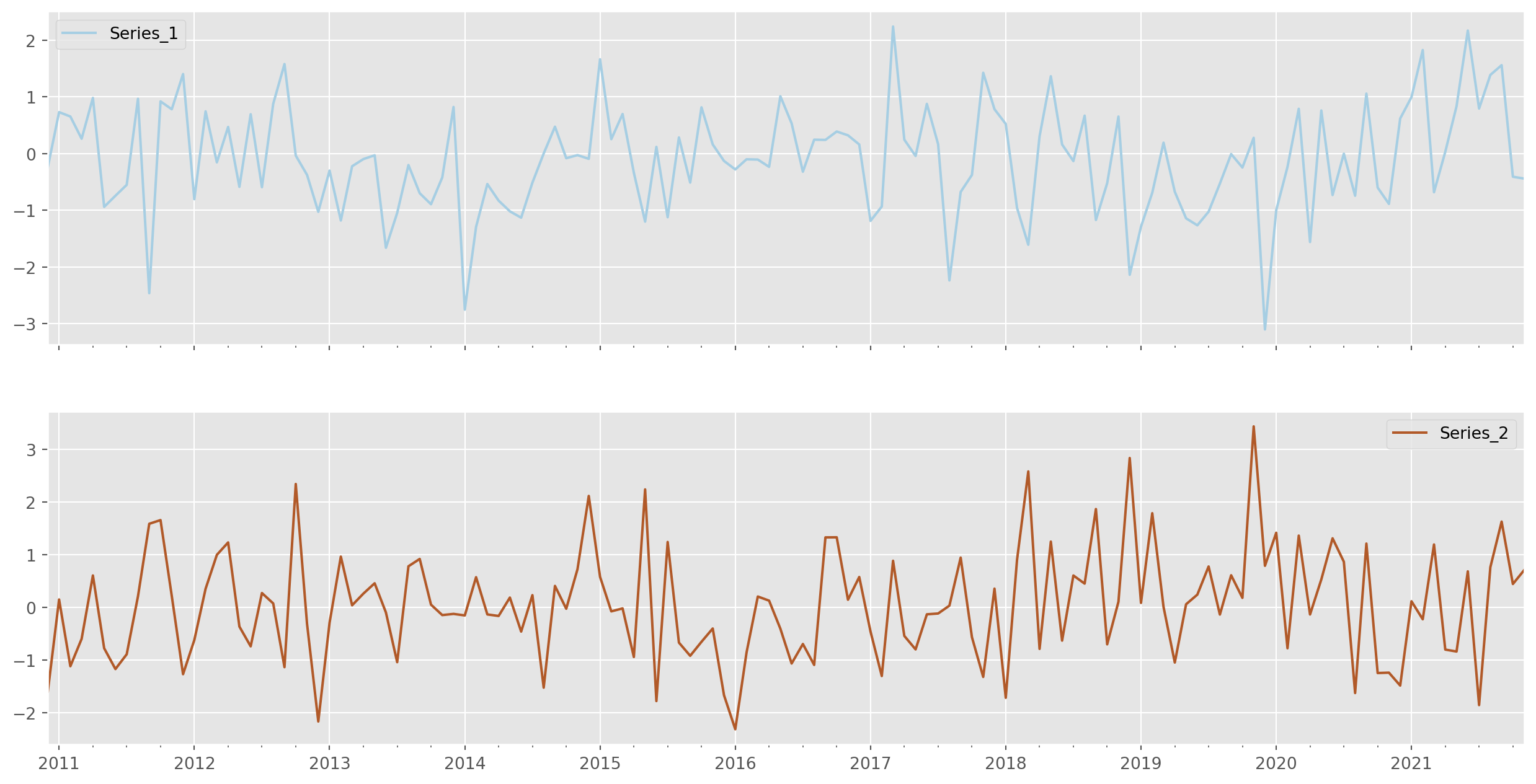
Upsampling
Upsampling is a technique for increasing the frequency or filling missing observations of a time series.
As an example, retrieve some real time series.
tesla_stockp = yf.download(tickers=["TSLA"], start="2018-1-1", end=dt.datetime.today())[*********************100%***********************] 1 of 1 completedtesla_stockp.tail()| Open | High | Low | Close | Adj Close | Volume | |
|---|---|---|---|---|---|---|
| Date | ||||||
| 2024-10-21 | 218.899994 | 220.479996 | 215.729996 | 218.850006 | 218.850006 | 47329000 |
| 2024-10-22 | 217.309998 | 218.220001 | 215.259995 | 217.970001 | 217.970001 | 43268700 |
| 2024-10-23 | 217.130005 | 218.720001 | 212.110001 | 213.649994 | 213.649994 | 80938900 |
| 2024-10-24 | 244.679993 | 262.119995 | 242.649994 | 260.480011 | 260.480011 | 204491900 |
| 2024-10-25 | 256.010010 | 269.489990 | 255.320007 | 269.190002 | 269.190002 | 161061400 |
tesla_stockp.loc["2019-11-15":, ["Close"]].plot(
    figsize=(12, 6), title="Tesla Stock Price 2019-11 to 2021-08"
)
plt.show()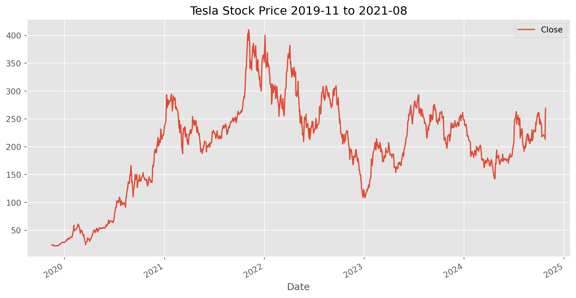
Notice that weekends and holidays are excluded from the index, which means there won’t be any n/a on those days, such as 2018-01-06 and 2018-01-06 as below.
tesla_stockp.head(10)| Open | High | Low | Close | Adj Close | Volume | |
|---|---|---|---|---|---|---|
| Date | ||||||
| 2018-01-02 | 20.799999 | 21.474001 | 20.733334 | 21.368668 | 21.368668 | 65283000 |
| 2018-01-03 | 21.400000 | 21.683332 | 21.036667 | 21.150000 | 21.150000 | 67822500 |
| 2018-01-04 | 20.858000 | 21.236668 | 20.378668 | 20.974667 | 20.974667 | 149194500 |
| 2018-01-05 | 21.108000 | 21.149332 | 20.799999 | 21.105333 | 21.105333 | 68868000 |
| 2018-01-08 | 21.066668 | 22.468000 | 21.033333 | 22.427334 | 22.427334 | 147891000 |
| 2018-01-09 | 22.344000 | 22.586666 | 21.826668 | 22.246000 | 22.246000 | 107199000 |
| 2018-01-10 | 22.146667 | 22.466667 | 22.000000 | 22.320000 | 22.320000 | 64648500 |
| 2018-01-11 | 22.349333 | 22.987333 | 22.217333 | 22.530001 | 22.530001 | 99682500 |
| 2018-01-12 | 22.575333 | 22.694000 | 22.244667 | 22.414667 | 22.414667 | 72376500 |
| 2018-01-16 | 22.502666 | 23.000000 | 22.320000 | 22.670668 | 22.670668 | 97114500 |
Upsampling to including non-trade days, such as weekends and holidays.
tesla_stockp.asfreq("D").head(10)| Open | High | Low | Close | Adj Close | Volume | |
|---|---|---|---|---|---|---|
| Date | ||||||
| 2018-01-02 | 20.799999 | 21.474001 | 20.733334 | 21.368668 | 21.368668 | 65283000.0 |
| 2018-01-03 | 21.400000 | 21.683332 | 21.036667 | 21.150000 | 21.150000 | 67822500.0 |
| 2018-01-04 | 20.858000 | 21.236668 | 20.378668 | 20.974667 | 20.974667 | 149194500.0 |
| 2018-01-05 | 21.108000 | 21.149332 | 20.799999 | 21.105333 | 21.105333 | 68868000.0 |
| 2018-01-06 | NaN | NaN | NaN | NaN | NaN | NaN |
| 2018-01-07 | NaN | NaN | NaN | NaN | NaN | NaN |
| 2018-01-08 | 21.066668 | 22.468000 | 21.033333 | 22.427334 | 22.427334 | 147891000.0 |
| 2018-01-09 | 22.344000 | 22.586666 | 21.826668 | 22.246000 | 22.246000 | 107199000.0 |
| 2018-01-10 | 22.146667 | 22.466667 | 22.000000 | 22.320000 | 22.320000 | 64648500.0 |
| 2018-01-11 | 22.349333 | 22.987333 | 22.217333 | 22.530001 | 22.530001 | 99682500.0 |
In the plot below, you can notice some obvious gaps now, because we have inserted weekend indices with n/a.
tesla_stockp.asfreq("D").loc["2019-11-15":, ["Close"]].plot(
    figsize=(12, 6), title="Tesla Stock Price 2019-11 to 2021-08"
)
plt.show()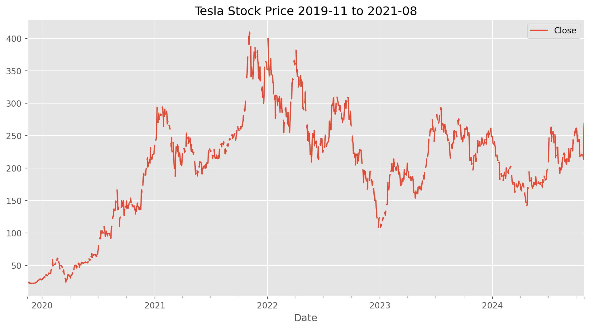
Compare Each Years Data
reset_index can drop index, so we can align each year as parallel columns.
tesla_prices = pd.DataFrame()  # placeholder dataframe
for year in ["2018", "2019", "2020", "2021"]:
    price_per_year = tesla_stockp.loc[year, ["Close"]].reset_index(drop=True)
    price_per_year.rename(columns={"Close": year + " close"}, inplace=True)
    tesla_prices = pd.concat([tesla_prices, price_per_year], axis=1)

tesla_prices.head()| 2018 close | 2019 close | 2020 close | 2021 close | |
|---|---|---|---|---|
| 0 | 21.368668 | 20.674667 | 28.684000 | 243.256668 |
| 1 | 21.150000 | 20.024000 | 29.534000 | 245.036667 |
| 2 | 20.974667 | 21.179333 | 30.102667 | 251.993332 |
| 3 | 21.105333 | 22.330667 | 31.270666 | 272.013336 |
| 4 | 22.427334 | 22.356667 | 32.809334 | 293.339996 |
Here we can visually compare the performance of each year.
tesla_prices.plot(figsize=(12, 6), title="Tesla Stock Price Comparison")
plt.show()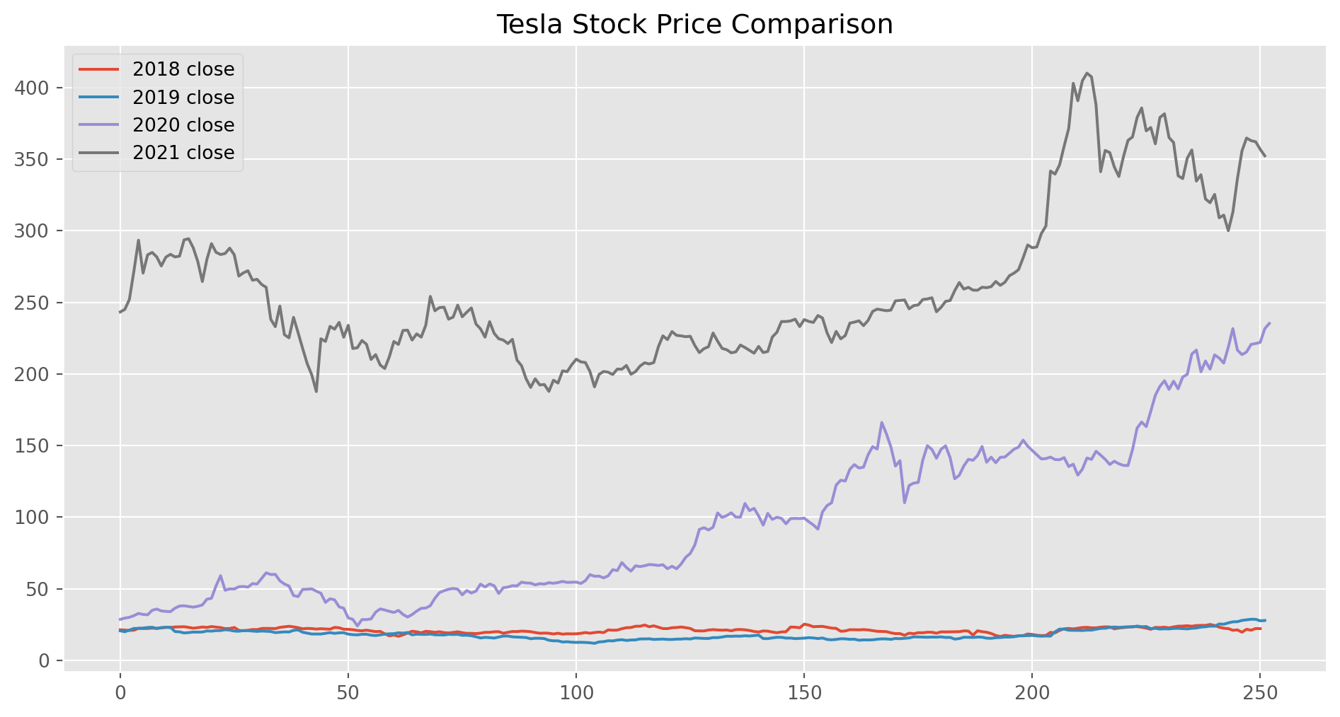
Resampling
.asfreq can change the series the frequency, here we use a keyword W-Wed to change the series to weekly Wednesday.
tesla_stockp["Close"].asfreq("W-Wed").tail()Date
2024-09-25 257.019989
2024-10-02 249.020004
2024-10-09 241.050003
2024-10-16 221.330002
2024-10-23 213.649994
Freq: W-WED, Name: Close, dtype: float64tesla_stockp["Close"].asfreq("W-Wed").plot(figsize=(12, 6))
plt.show()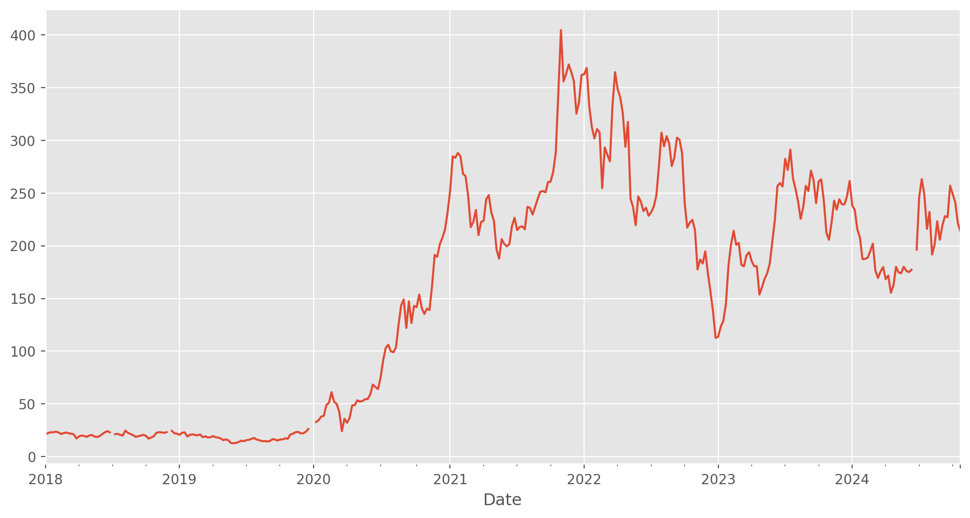
If we use M frequency, pandas will pick the last day of each month.
tesla_stockp["Close"].asfreq("M").plot(figsize=(12, 6))
plt.show()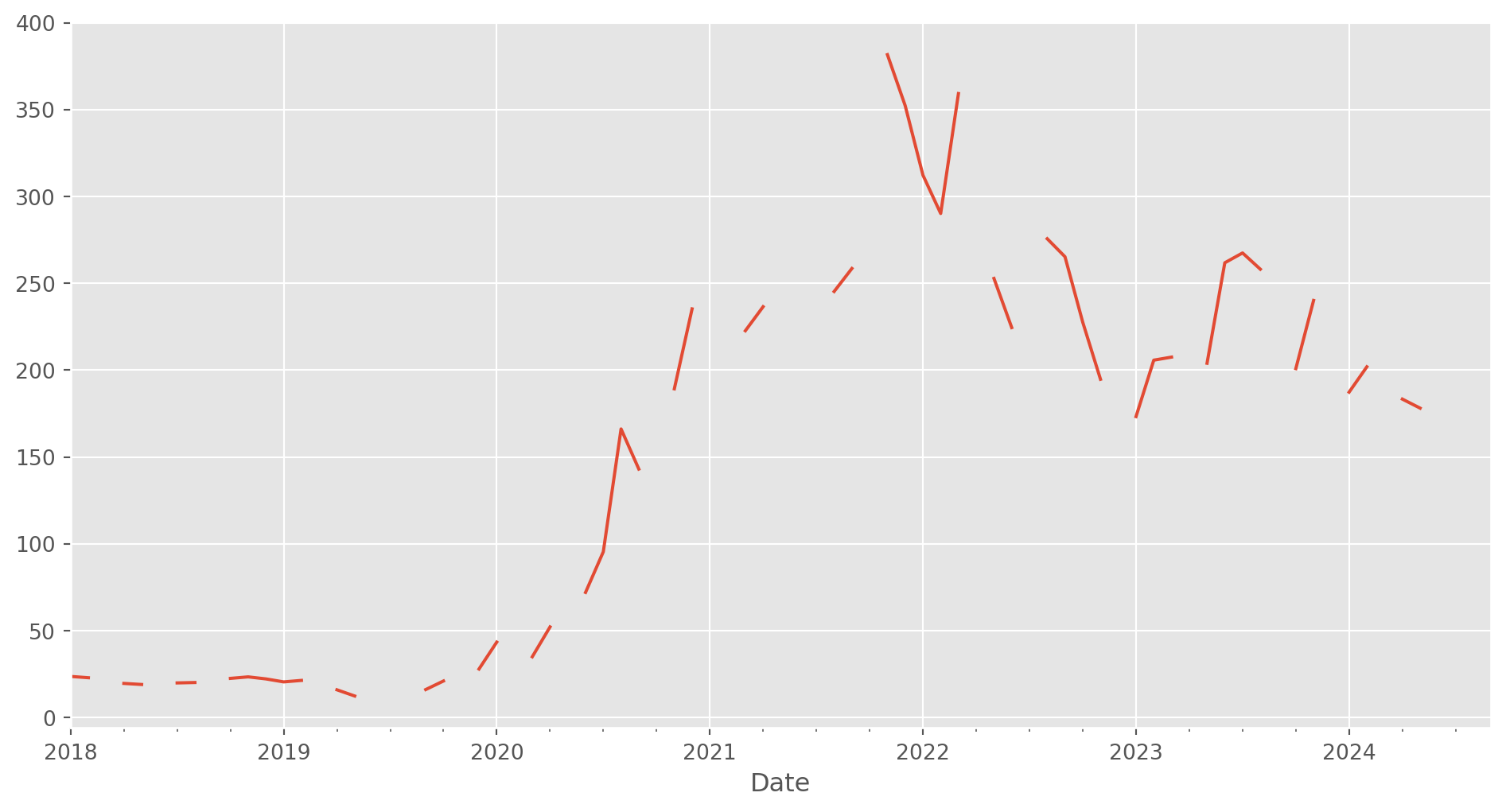
But it turns out that many days at the end of month are weekend, which causes multiple n/a values and breaks in the plots.
However method='bfill' can fill the empty observation with previous one.
tesla_stockp["Close"].asfreq("M", method="bfill").plot(figsize=(12, 6))
plt.show()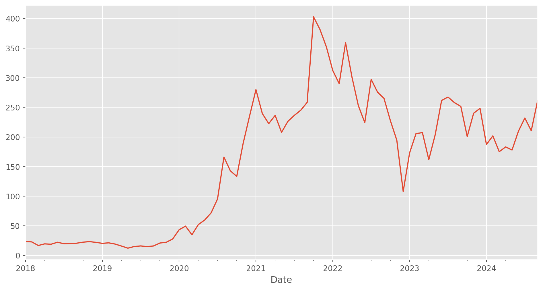
Lagged Variable
Lagged variable usually denoted as \(y_{t-i}\) where \(i \in \{1, 2, 3,...\}\), in practice, we move the data at \(t-i\) to current period. The example of \(y_{t-1}\) is added as Lag_1 column.
Pick the close price then shift \(1\) period backward. And gross daily change would be straightforward now.
tesla_stockp["Lag_1"] = tesla_stockp["Close"].shift()
tesla_stockp["Daily Change"] = tesla_stockp["Close"].div(tesla_stockp["Lag_1"])tesla_stockp.head()| Open | High | Low | Close | Adj Close | Volume | Lag_1 | Daily Change | |
|---|---|---|---|---|---|---|---|---|
| Date | ||||||||
| 2018-01-02 | 20.799999 | 21.474001 | 20.733334 | 21.368668 | 21.368668 | 65283000 | NaN | NaN |
| 2018-01-03 | 21.400000 | 21.683332 | 21.036667 | 21.150000 | 21.150000 | 67822500 | 21.368668 | 0.989767 |
| 2018-01-04 | 20.858000 | 21.236668 | 20.378668 | 20.974667 | 20.974667 | 149194500 | 21.150000 | 0.991710 |
| 2018-01-05 | 21.108000 | 21.149332 | 20.799999 | 21.105333 | 21.105333 | 68868000 | 20.974667 | 1.006230 |
| 2018-01-08 | 21.066668 | 22.468000 | 21.033333 | 22.427334 | 22.427334 | 147891000 | 21.105333 | 1.062638 |
tesla_stockp["Daily Change"].plot(figsize=(12, 5))
plt.show()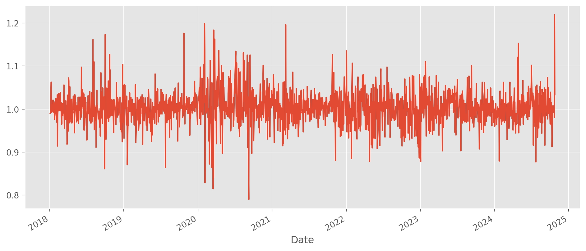
You can also plot histogram.
ax = tesla_stockp["Daily Change"].plot.hist(bins=60, alpha=0.5, figsize=(12, 5))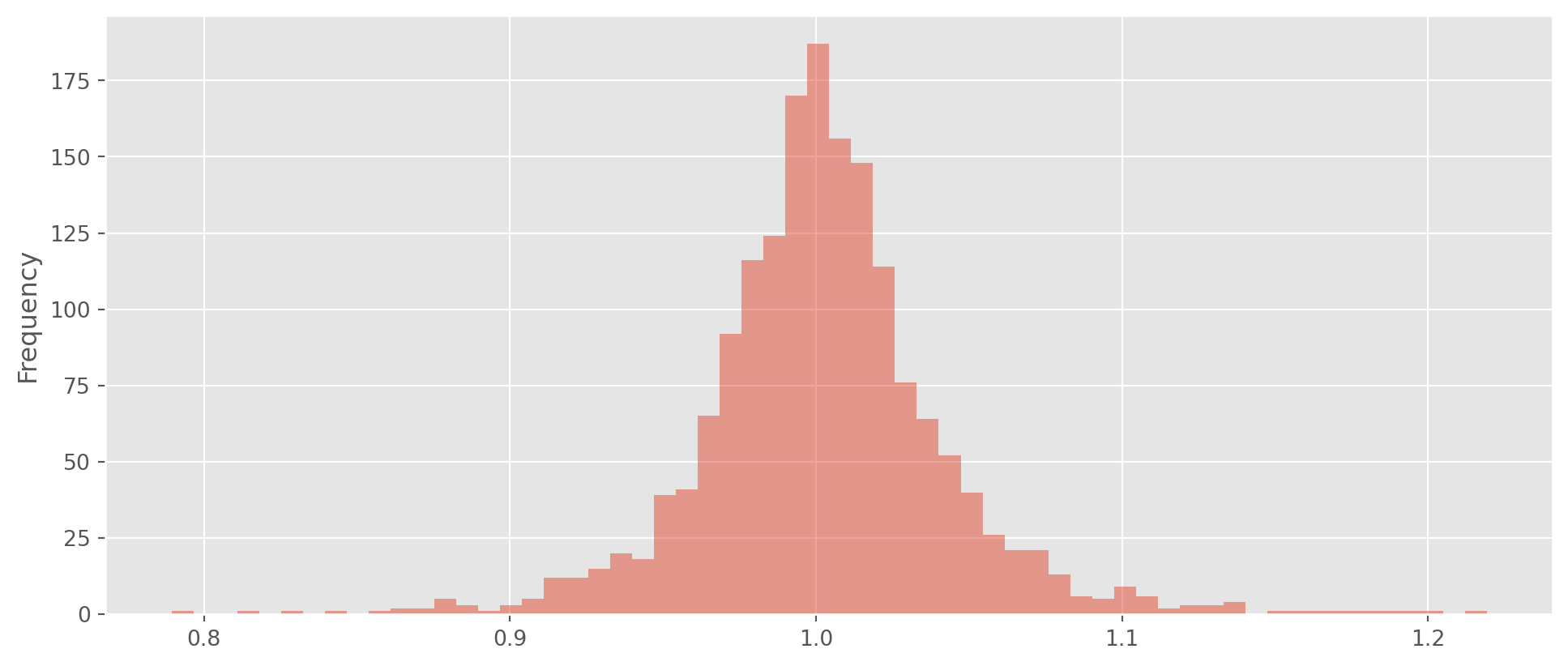
Growth Rate
The daily change rate or rate of change has a convenient computing method in Pandas.
tesla_stockp["change_pct"] = tesla_stockp["Close"].pct_change()tesla_stockp["change_pct"].plot(figsize=(12, 5))
plt.show()
You can also choose the period.
tesla_stockp["change_pct_daily"] = tesla_stockp["Close"].pct_change()
tesla_stockp["change_pct_monthly"] = tesla_stockp["Close"].pct_change(periods=30)
tesla_stockp["change_pct_yearly"] = tesla_stockp["Close"].pct_change(periods=360)
tesla_stockp[["change_pct_daily", "change_pct_monthly", "change_pct_yearly"]].plot(
    subplots=True, figsize=(12, 9)
)
plt.show()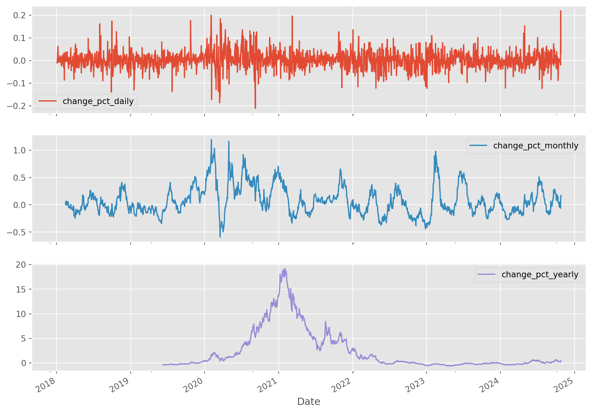
Price Normalization
Normalization is a very common practice to compare data which have different level of values. It transforms the data into the same initial value for easy comparison.
Let’s import some data.
# SP500, Gold, Crude oil, Gold, Bitcoin, Nikkei 225
assets_tickers = ["^GSPC", "GC=F", "CL=F", "BTC-USD", "^N225"]
legends = ["SP500", "Gold", "Crude oil", "Gold", "Bitcoin", "Nikkei 225"]
start_date = "2022-1-1"
end_date = dt.datetime.today()
assets_price = yf.download(tickers=assets_tickers, start=start_date, end=end_date)
[ 0% ][******************* 40% ] 2 of 5 completed[**********************60%**** ] 3 of 5 completed[**********************80%************* ] 4 of 5 completed[*********************100%***********************] 5 of 5 completedBasically, the essential step is to divide all observations by the first one, whether to multiply \(100\) is largely optional.
Here in the example, we normalize all data to start from \(100\).
assets_price = assets_price["Close"].dropna()normalized_prices = assets_price.div(assets_price.iloc[0]).mul(100)price_plot = normalized_prices.plot(figsize=(12, 5))
price_plot.legend(legends)
plt.show()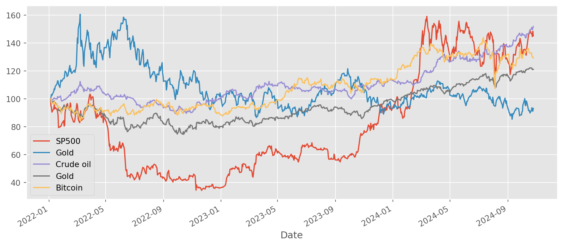
Correlation
Seaborn has convenient functions for plotting correlation.
# SP500, Gold, Crude oil, Gold, Bitcoin, Nikkei 225
assets_tickers = ["^GSPC", "GC=F", "CL=F", "BTC-USD", "^N225"]
legends = ["SP500", "Gold", "Crude oil", "Gold", "Bitcoin", "Nikkei 225"]
start_date = "2020-1-1"
end_date = dt.datetime.today()
assets_price = yf.download(tickers=assets_tickers, start=start_date, end=end_date)
[ 0% ][******************* 40% ] 2 of 5 completed[**********************60%**** ] 3 of 5 completed[**********************80%************* ] 4 of 5 completed[*********************100%***********************] 5 of 5 completedassets_close = assets_price["Close"]
assets_close.columns = ["SP500", "Crude oil", "Gold", "Bitcoin", "Nikkei 225"]sns.jointplot(x="Nikkei 225", y="SP500", data=assets_close.pct_change())
plt.show()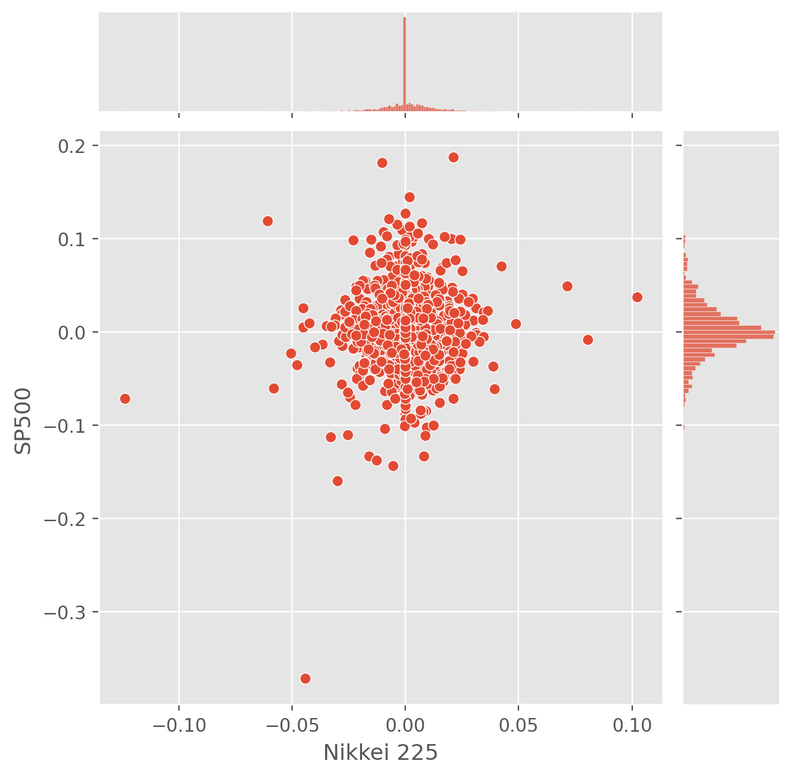
.corr() can produce a correlation matrix, to visualize with color, simply import it in seaborn’s heatmap.
assets_corr = assets_close.pct_change().corr()
assets_corr| SP500 | Crude oil | Gold | Bitcoin | Nikkei 225 | |
|---|---|---|---|---|---|
| SP500 | 1.000000 | 0.067041 | 0.121548 | 0.351753 | 0.063031 |
| Crude oil | 0.067041 | 1.000000 | 0.044765 | 0.130733 | 0.072898 |
| Gold | 0.121548 | 0.044765 | 1.000000 | 0.128936 | 0.078203 |
| Bitcoin | 0.351753 | 0.130733 | 0.128936 | 1.000000 | 0.222949 |
| Nikkei 225 | 0.063031 | 0.072898 | 0.078203 | 0.222949 | 1.000000 |
sns.heatmap(assets_corr, annot=True, cmap=sns.cm.rocket_r, annot_kws={"size": 12})
plt.show()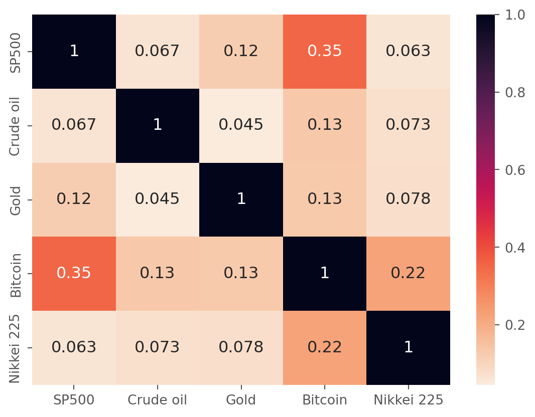
Furthermore, clustermap can organize similar data by similarity, which brings more insight into the data set.
sns.clustermap(assets_corr, cmap=sns.cm.rocket_r)
plt.show()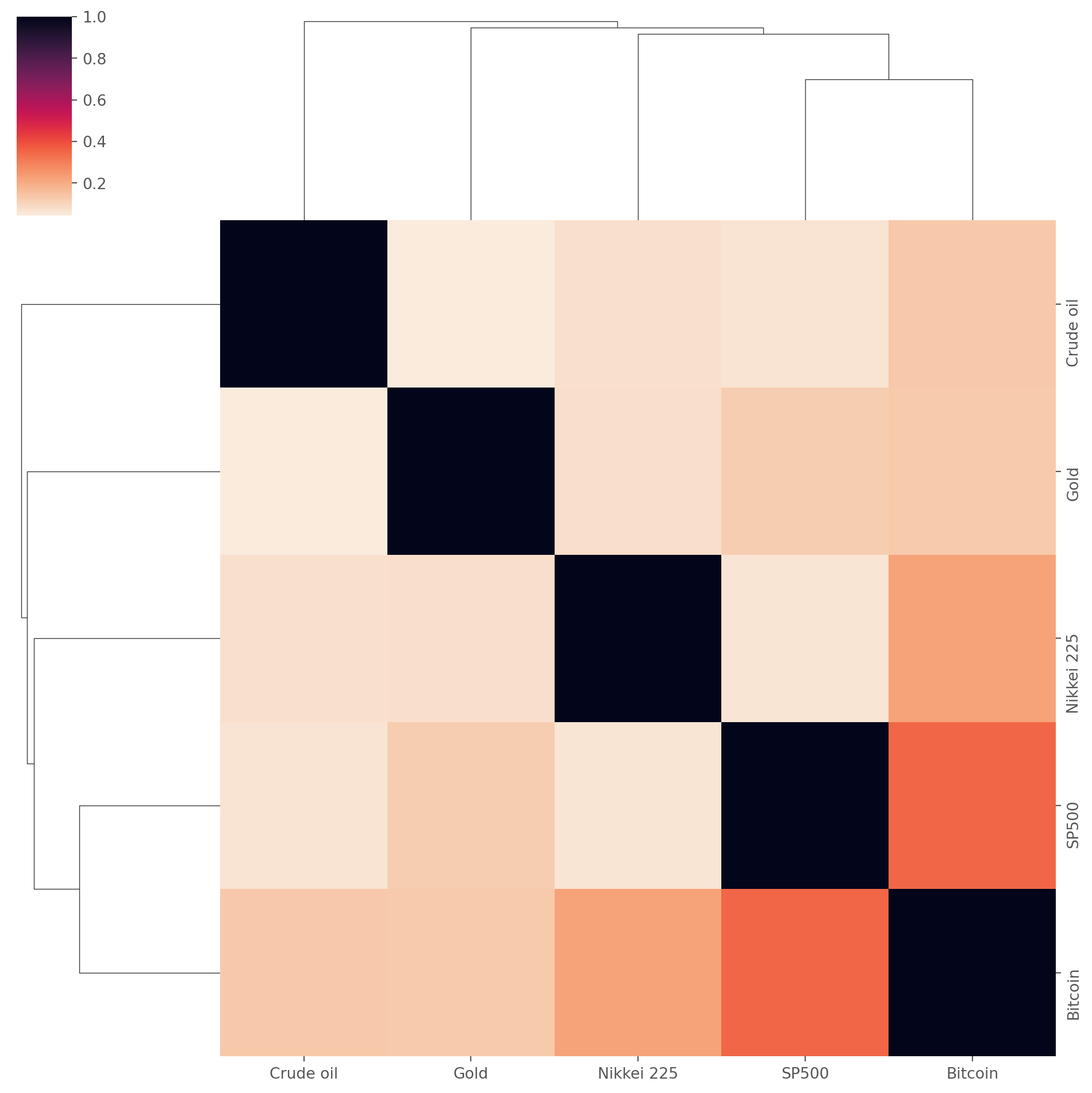
It would be more meaningful to compare the rate of change sometimes.
df = yf.download(["JPM", "^RUT"], start)["Close"]
df.columns = ["JPM", "Russel2000"]
df_change = df.pct_change()
df_change.columns = ["JPM_ret", "Russel2000_ret"]
df_change.head()
[ 0% ][*********************100%***********************] 2 of 2 completed| JPM_ret | Russel2000_ret | |
|---|---|---|
| Date | ||
| 2018-01-02 00:00:00+00:00 | NaN | NaN |
| 2018-01-03 00:00:00+00:00 | 0.001019 | 0.001658 |
| 2018-01-04 00:00:00+00:00 | 0.009069 | 0.002022 |
| 2018-01-05 00:00:00+00:00 | -0.006420 | 0.002758 |
| 2018-01-08 00:00:00+00:00 | 0.001477 | 0.001154 |
sns.relplot(x="JPM_ret", y="Russel2000_ret", data=df_change)
plt.show()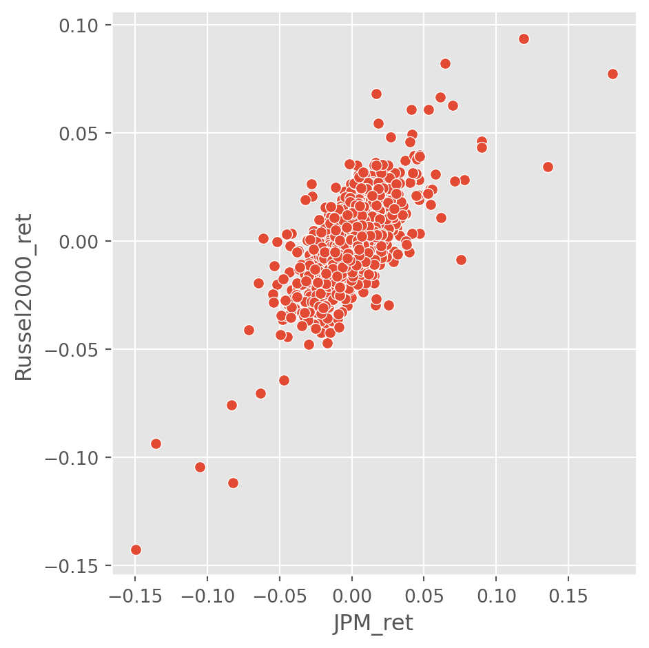
Changing Data Frequency
Here is how to create an index labeled the end of each month.
start = "2021-1-15"
end = "2021-12-20"
dates = pd.date_range(start=start, end=end, freq="M")
dates
DatetimeIndex(['2021-01-31', '2021-02-28', '2021-03-31', '2021-04-30',
'2021-05-31', '2021-06-30', '2021-07-31', '2021-08-31',
'2021-09-30', '2021-10-31', '2021-11-30'],
dtype='datetime64[ns]', freq='ME')monthly = pd.Series(data=np.arange(len(dates)), index=dates)
monthly2021-01-31 0
2021-02-28 1
2021-03-31 2
2021-04-30 3
2021-05-31 4
2021-06-30 5
2021-07-31 6
2021-08-31 7
2021-09-30 8
2021-10-31 9
2021-11-30 10
Freq: ME, dtype: int64At the end of each week, i.e. Sunday. (Ignore the old fashion of regarding Sunday as the first day of the week.)
weekly_dates = pd.date_range(start=start, end=end, freq="W")
weekly_dates
DatetimeIndex(['2021-01-17', '2021-01-24', '2021-01-31', '2021-02-07',
'2021-02-14', '2021-02-21', '2021-02-28', '2021-03-07',
'2021-03-14', '2021-03-21', '2021-03-28', '2021-04-04',
'2021-04-11', '2021-04-18', '2021-04-25', '2021-05-02',
'2021-05-09', '2021-05-16', '2021-05-23', '2021-05-30',
'2021-06-06', '2021-06-13', '2021-06-20', '2021-06-27',
'2021-07-04', '2021-07-11', '2021-07-18', '2021-07-25',
'2021-08-01', '2021-08-08', '2021-08-15', '2021-08-22',
'2021-08-29', '2021-09-05', '2021-09-12', '2021-09-19',
'2021-09-26', '2021-10-03', '2021-10-10', '2021-10-17',
'2021-10-24', '2021-10-31', '2021-11-07', '2021-11-14',
'2021-11-21', '2021-11-28', '2021-12-05', '2021-12-12',
'2021-12-19'],
dtype='datetime64[ns]', freq='W-SUN')Conform the data with new index. bfill and ffill, meaning fill backward and forward, will be handy.
Here we transform the monthly frequency data into weekly, the NaN will be filled by one of filling method above.
monthly.reindex(weekly_dates).head(10) # without fill2021-01-17 NaN
2021-01-24 NaN
2021-01-31 0.0
2021-02-07 NaN
2021-02-14 NaN
2021-02-21 NaN
2021-02-28 1.0
2021-03-07 NaN
2021-03-14 NaN
2021-03-21 NaN
Freq: W-SUN, dtype: float64# bfill can fill past dates with the most current available ones
monthly.reindex(weekly_dates, method="bfill").head(10)2021-01-17 0.0
2021-01-24 0.0
2021-01-31 0.0
2021-02-07 1.0
2021-02-14 1.0
2021-02-21 1.0
2021-02-28 1.0
2021-03-07 2.0
2021-03-14 2.0
2021-03-21 2.0
Freq: W-SUN, dtype: float64# compare with bfill
monthly.reindex(weekly_dates, method="ffill").head(10)2021-01-17 NaN
2021-01-24 NaN
2021-01-31 0.0
2021-02-07 0.0
2021-02-14 0.0
2021-02-21 0.0
2021-02-28 1.0
2021-03-07 1.0
2021-03-14 1.0
2021-03-21 1.0
Freq: W-SUN, dtype: float64Unemployment data are generally published every month.
df_unempl = pdr.data.DataReader(
    name="UNRATE", data_source="fred", start="2000-1-1", end=dt.date.today()
)
df_unempl.columns = ["Unemployment_Rate"]
df_unempl.plot(figsize=(12, 5))
plt.show()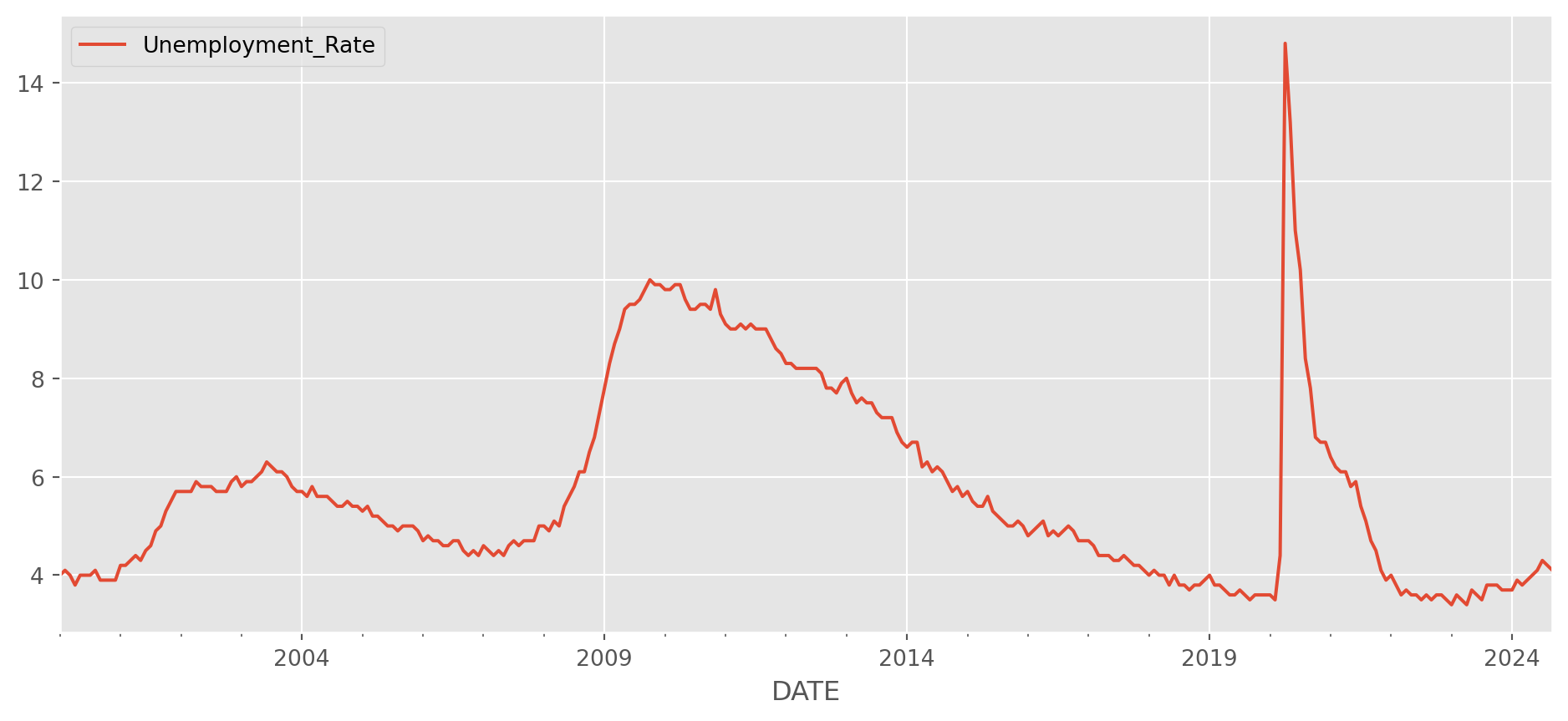
Because it is a monthly series, the exactly date of publication doesn’t matter, so all the data are indexed on the first day of each month.
df_unempl.head()| Unemployment_Rate | |
|---|---|
| DATE | |
| 2000-01-01 | 4.0 |
| 2000-02-01 | 4.1 |
| 2000-03-01 | 4.0 |
| 2000-04-01 | 3.8 |
| 2000-05-01 | 4.0 |
Change the frequency to weekly data, the missing values will be filled by existing values.
df_unempl_bfill = df_unempl.asfreq("W", method="bfill")
df_unempl_ffill = df_unempl.asfreq("W", method="ffill")
df_unempl_concat = pd.concat([df_unempl_bfill, df_unempl_ffill], axis=1)
df_unempl_concat.columns = ["unemp_rate_bfilled_weekly", "unemp_rate_ffilled_weekly"]
Compare the filled data.
df_unempl_concat.plot(figsize=(16, 6))
plt.show()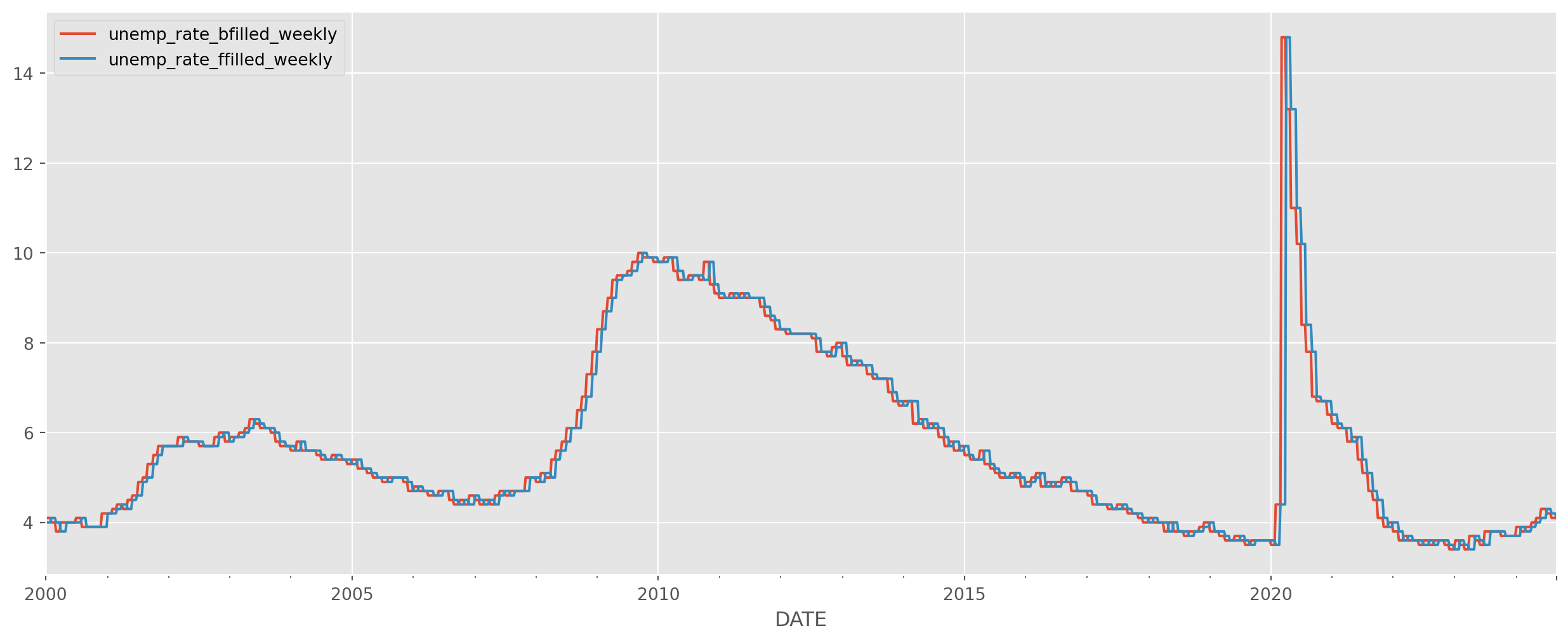
Interpolation
Interpolation is a more sensible way to fill the NaN in data, it could either fill linearly or nonlinearly.
Import the labor participation rate, which is a monthly series.
lab_part = pdr.data.DataReader(
    name="CIVPART", data_source="fred", start="2010-1-1", end=dt.date.today()
)
lab_part.columns = ["Labor_Participation_Rate"]
lab_part.plot(figsize=(12, 5))
plt.show()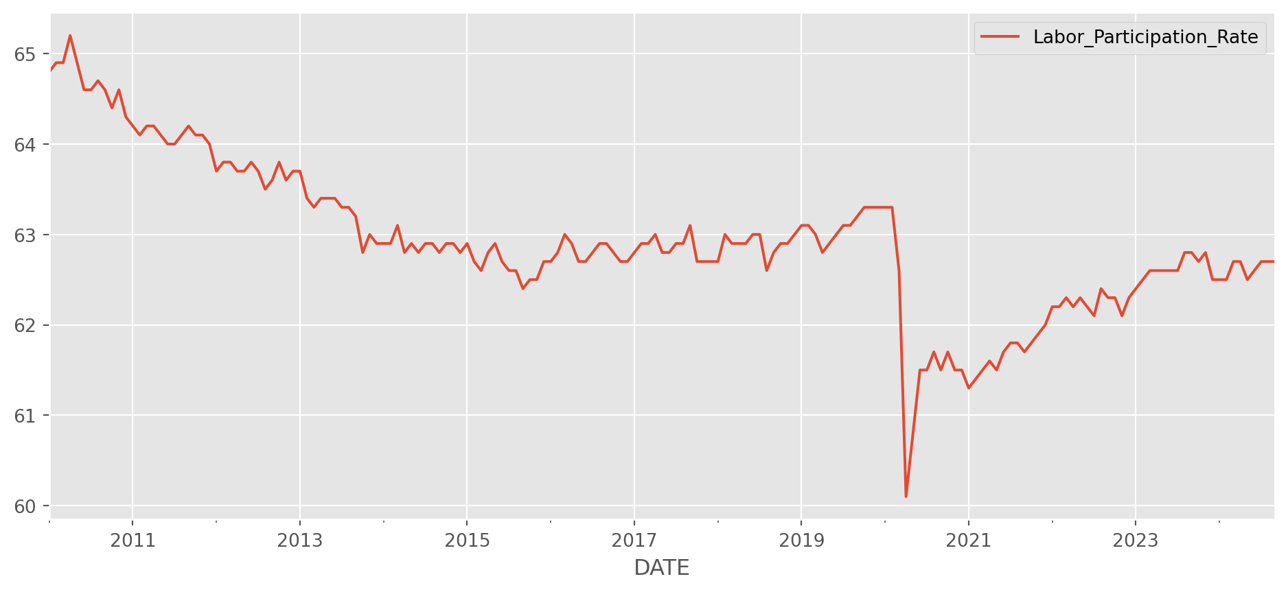
To transform the monthly series into a daily series, we pick the start and end date first.
daily_dates = pd.date_range(
    start=lab_part.index.min(), end=lab_part.index.max(), freq="D"
)
Reindex the monthly series as daily series. Make one forward fill and one interpolation, compare them.
lab_part_daily = lab_part.reindex(daily_dates)
lab_part_daily["forward_fill"] = lab_part_daily["Labor_Participation_Rate"].ffill()
lab_part_daily["interpolation"] = lab_part_daily[
    "Labor_Participation_Rate"
].interpolate() # this is exactly the plot abovelab_part_daily.plot(figsize=(16, 6))
plt.show()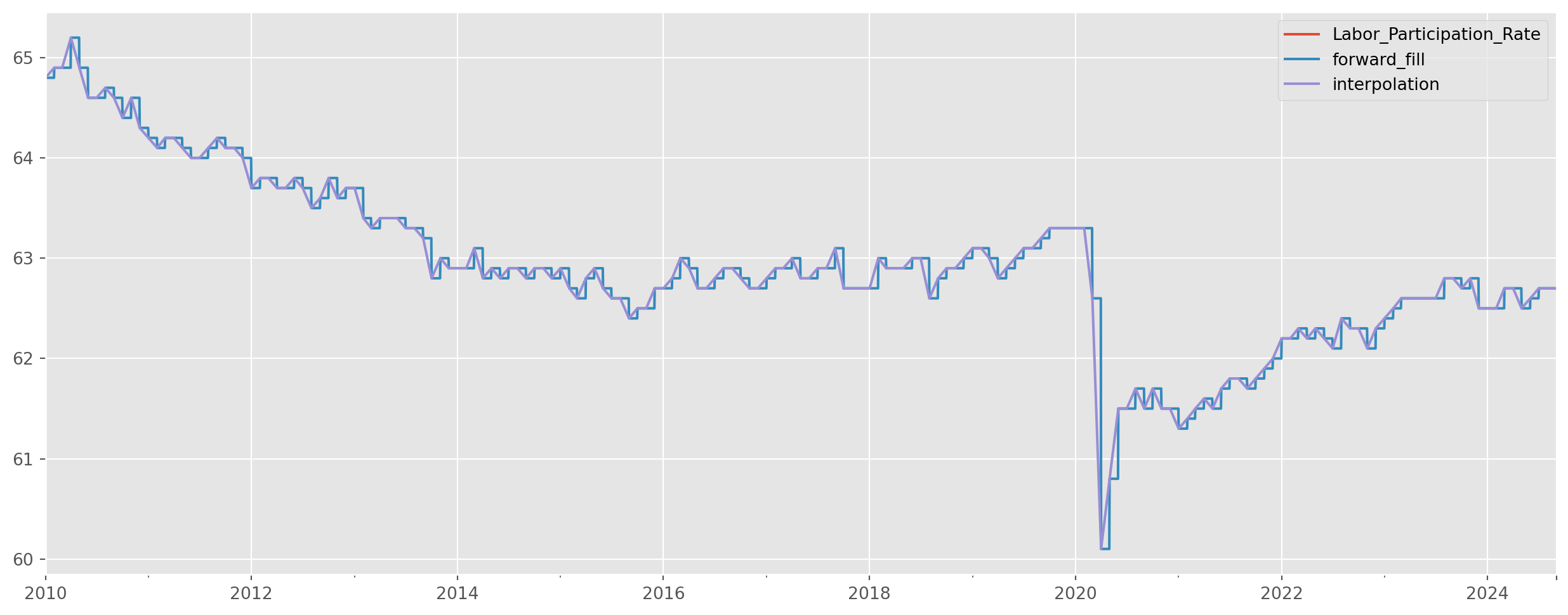
Resampling Plot
Here is an example of down-sampling the frequency of series. Let’s import 10y yield and crude oil price.
df = pdr.data.DataReader(
    name=["DFII10", "DCOILBRENTEU"],
    data_source="fred",
    start="2010-1-1",
    end=dt.date.today(),
)
df.columns = ["10y_TB_yield", "Crude_oil"]Draw plot with twin axes.
ax = df.plot(secondary_y="10y_TB_yield", figsize=(12, 5))
plt.show()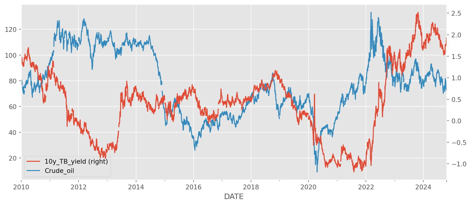
Please note that df.resample('M') is an object, not a series. Use the mean value as the monthly data.
ax = df.resample("M").mean().plot(secondary_y="10y_TB_yield", figsize=(16, 7))
plt.show()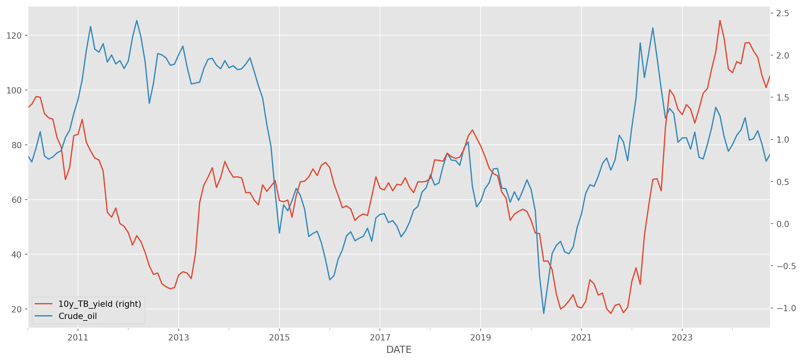
ax = df.resample("A").mean().plot(secondary_y="10y_TB_yield", figsize=(16, 7))
plt.show()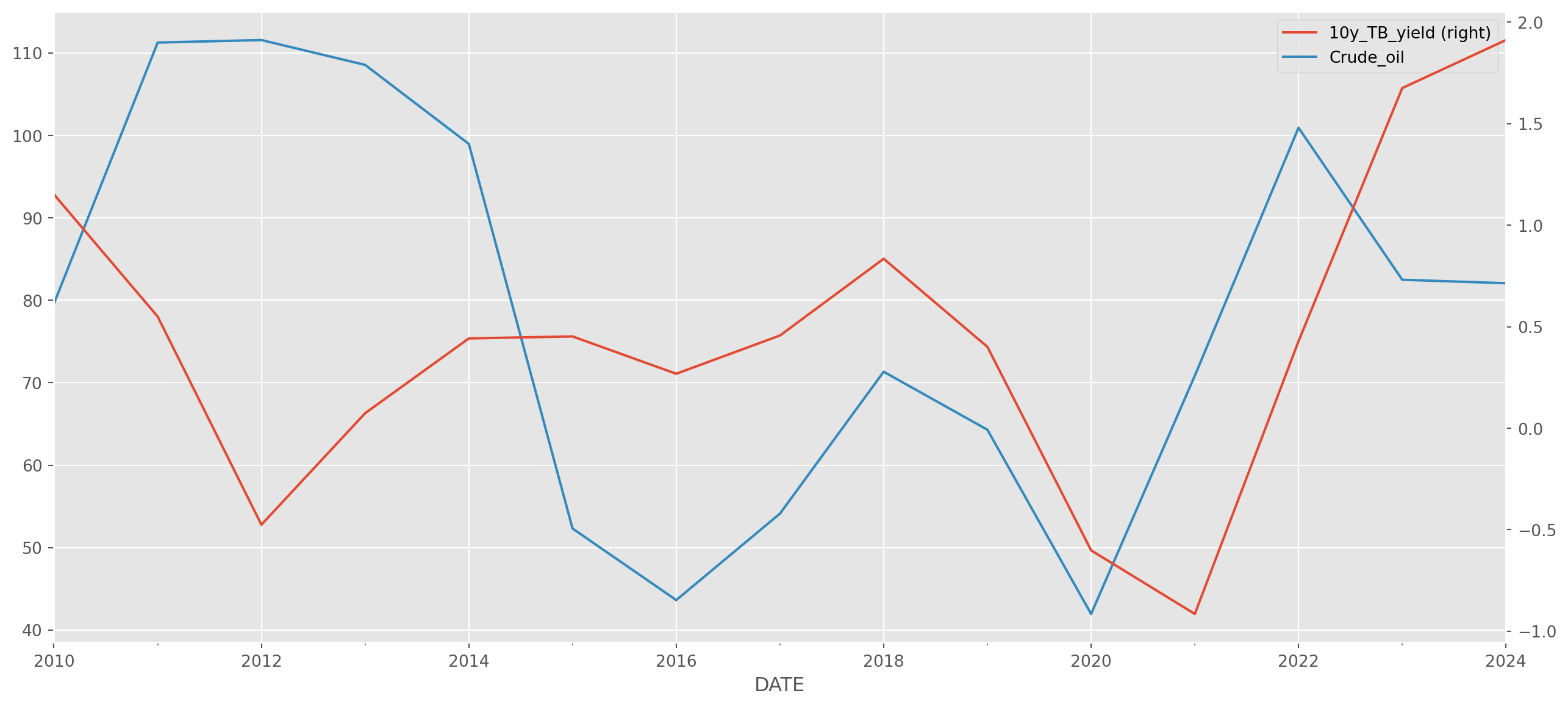
If you don’t want the monthly mean, you can pick the first or last observation as the monthly data.
df.resample("M").first().head()| 10y_TB_yield | Crude_oil | |
|---|---|---|
| DATE | ||
| 2010-01-31 | 1.47 | 79.05 |
| 2010-02-28 | 1.29 | 71.58 |
| 2010-03-31 | 1.46 | 76.07 |
| 2010-04-30 | 1.61 | 82.63 |
| 2010-05-31 | 1.32 | 88.09 |
df.resample("M").last().head()| 10y_TB_yield | Crude_oil | |
|---|---|---|
| DATE | ||
| 2010-01-31 | 1.30 | 71.20 |
| 2010-02-28 | 1.48 | 76.36 |
| 2010-03-31 | 1.60 | 80.37 |
| 2010-04-30 | 1.29 | 86.19 |
| 2010-05-31 | 1.32 | 73.00 |
Conform the Frequency Among Time Series
Let’s pick three series with different frequencies.
data_list = ["GDPC1", "SP500", "U2RATE"]
df = pdr.data.DataReader(
    name=data_list, data_source="fred", start="2021-1-1", end=dt.datetime.today()
)
df.columns = ["realGDP", "SP500", "unempRate"]Resample SP500 and Unemployment to quarterly change rate.
sp500_chrate_quarterly = df["SP500"].resample("QS").first().pct_change()
unempRate_quarterly = df["unempRate"].resample("QS").first().pct_change()
gdp_chrate = df["realGDP"].dropna().pct_change()
df_quarterly = pd.concat(
[gdp_chrate, sp500_chrate_quarterly, unempRate_quarterly], axis=1
)df_quarterly.plot(figsize=(12, 5))
plt.show()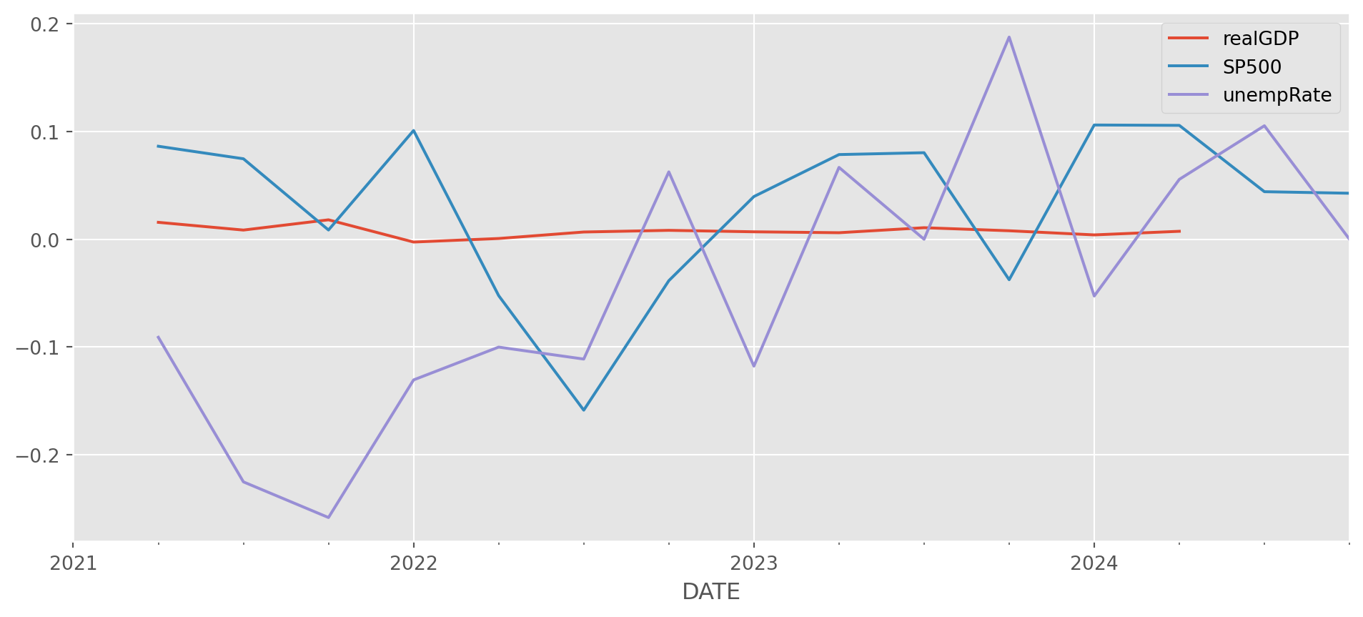
Apply Multiple Function
nk225 = pdr.data.DataReader(
    name="NIKKEI225", data_source="fred", start="2000-1-1", end=dt.datetime.today()
)
nk225_daily_return = nk225.pct_change()Here’s a fast method to calculate multiple statistics at once.
nk225_stats = nk225_daily_return.resample("W").agg(["mean", "median", "std"])nk225_stats.plot(figsize=(16, 6), alpha=0.7)
plt.show()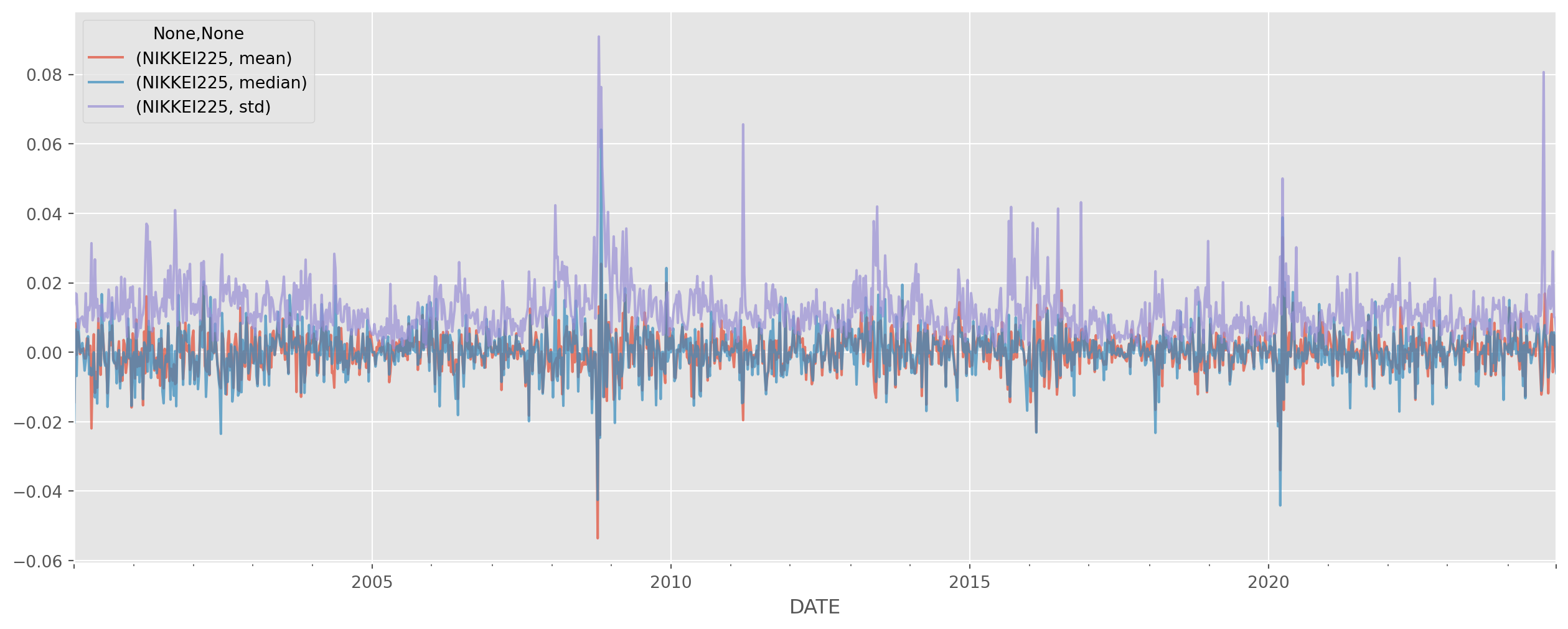
Rolling Window
Rolling window is one of most useful method for smoothing time series.
Let’s import USDJPY from Fred.
start_date = "2010-1-1"
end_date = dt.datetime.today()
usdjpy = pdr.data.DataReader(
    name="DEXJPUS", data_source="fred", start=start_date, end=end_date
).dropna()
Rolling window method can calculate moving average easily.
usdjpy["30D"] = usdjpy["DEXJPUS"].rolling(window="30D").mean()
usdjpy["60D"] = usdjpy["DEXJPUS"].rolling(window="60D").mean()
usdjpy["120D"] = usdjpy["DEXJPUS"].rolling(window="120D").mean()usdjpy.plot(figsize=(16, 10), grid=True, title="USDJPY and Rolling Means")
plt.show()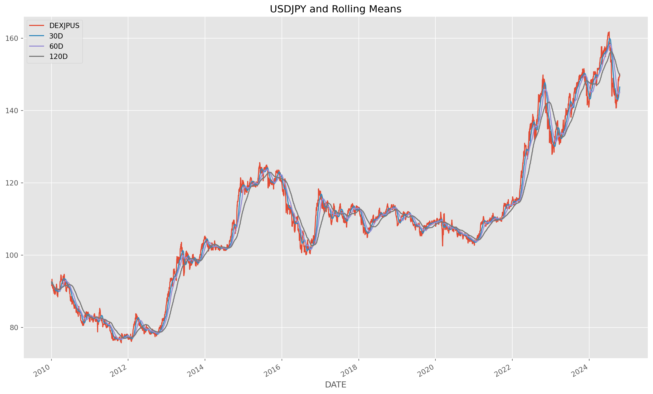
Rolling window doesn’t have to mean value, it could be any statistics too.
usdchf = pdr.data.DataReader(
    name="DEXSZUS", data_source="fred", start=start_date, end=end_date
).dropna()
rolling_stats = usdchf["DEXSZUS"].rolling(window=30).agg(["mean", "std"]).dropna()
usdchf = usdchf.join(rolling_stats)
usdchf.plot(subplots=True, figsize=(16, 12), grid=True)
plt.show()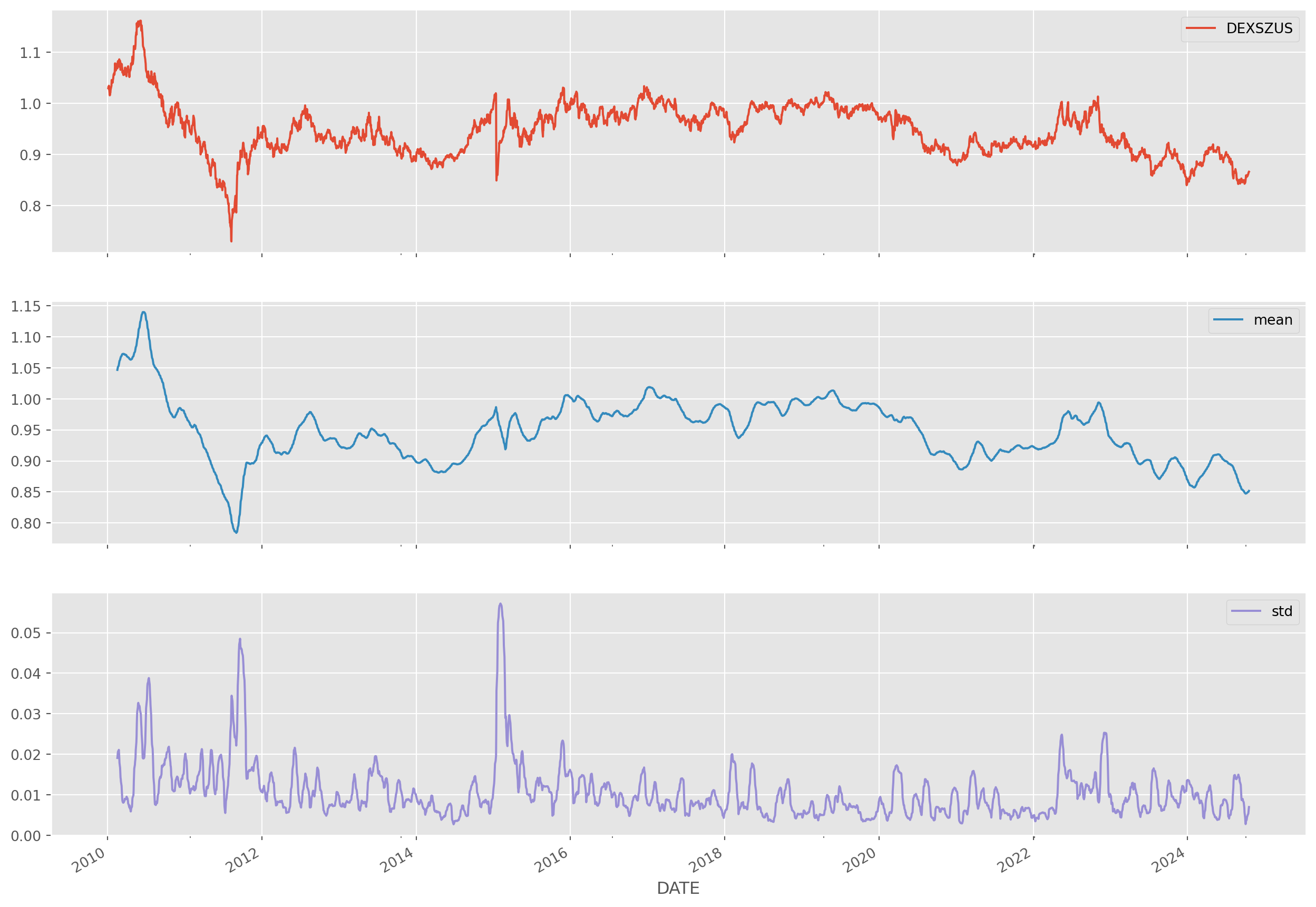
Rolling Window With Upper And Lower Bound
If we can calculate rolling standard deviation, we certainly can add it onto the original series or moving average to delineate a possibly boundary, this is the exact idea of Bollinger band.
usdjpy["mstd"] = usdjpy["DEXJPUS"].rolling(window=120).std()
usdjpy["MA"] = usdjpy["DEXJPUS"].rolling(window=120).mean()
usdjpy["upper"] = usdjpy["MA"] + usdjpy["mstd"] * 2
usdjpy["lower"] = usdjpy["MA"] - usdjpy["mstd"] * 2
usdjpy.iloc[:, 5:8].plot(figsize=(16, 6), title="120D rolling Window Bounds of USDJPY")
plt.show()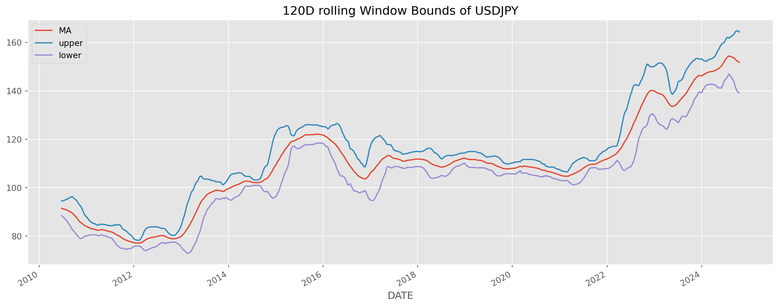
Rolling Quantile
Rolling quantiles are natural too.
dxy = pdr.data.DataReader(
    name="DTWEXBGS", data_source="fred", start=start_date, end=end_date
).dropna()
dxy.columns = ["DXY"]
dxy_rolling = dxy["DXY"].rolling(window=30)

dxy["q10"] = dxy_rolling.quantile(0.1)
dxy["q50"] = dxy_rolling.quantile(0.5)
dxy["q90"] = dxy_rolling.quantile(0.9)dxy.plot(grid=True, figsize=(16, 7))
plt.show()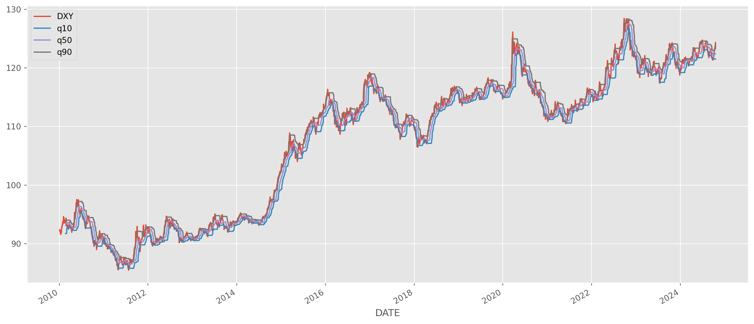
Cumulative Sum
The cumulative summation is the opposite operation of first order difference. However, don’t use this method to recover the data from first order difference, the result will never be the same as the original.
Take a look at this example.
sp500 = pdr.data.DataReader(
    name="SP500", data_source="fred", start="2010-1-1", end=dt.datetime.today()
)
sp500_diff = sp500.diff().dropna()first_day = sp500.first("D")
cumulative = pd.concat([first_day, sp500_diff]).cumsum()sp500.join(cumulative.add_suffix("_recovered")).plot(figsize=(12, 5), grid=True)
plt.show()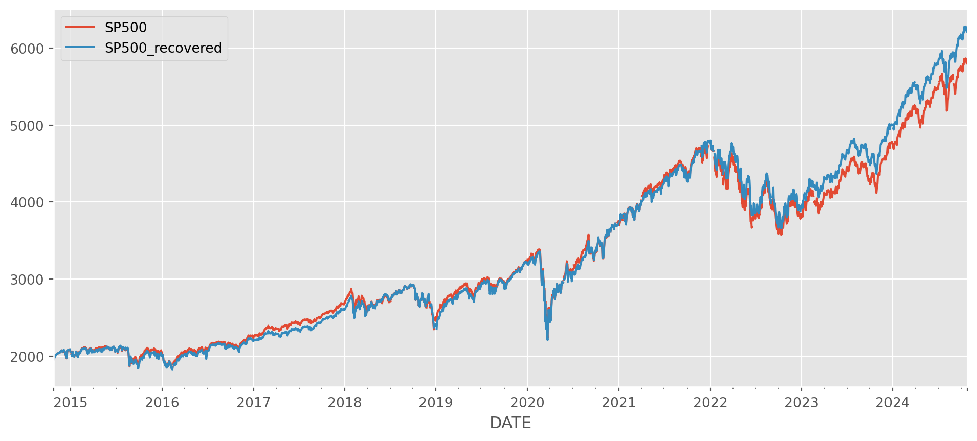
Cumulative Return
Choose your initial investment capital.
init_investment = 50000Retrieve Lululemon’s closing price.
lulu = yf.download(tickers="LULU", start="2010-1-1", end=dt.datetime.today())[
    "Close"
].to_frame()
[*********************100%***********************] 1 of 1 completedCalculate accumulative return with method cumprod().
lulu_cum_ret = lulu.pct_change().add(1).cumprod()(init_investment * lulu_cum_ret).plot(
figsize=(12, 6), grid=True, title="Lululemon Investment"
)
plt.show()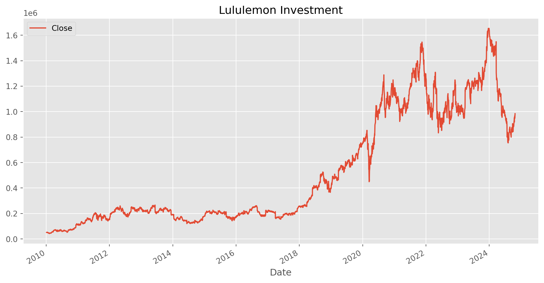
def multi_period_return(period_returns):
    return np.prod(period_returns + 1) - 1
# Lululemon, Nike, Adidas, Under Armour, Anta
stocks_list = ["LULU", "NKE", "ADS.F", "UA", "AS7.F"]
stocks = yf.download(tickers=stocks_list, start="2017-1-1", end=dt.datetime.today())[
"Close"
]
stocks.columns = ["Lululemon", "Nike", "Adidas", "Under Armour", "Anta"][ 0% ][******************* 40% ] 2 of 5 completed[**********************60%**** ] 3 of 5 completed[**********************80%************* ] 4 of 5 completed[*********************100%***********************] 5 of 5 completedstocks.pct_change().rolling(window="360D").apply(multi_period_return).mul(100).plot(
figsize=(12, 5), grid=True, title="Sports Brands Rolling Return"
)
plt.show()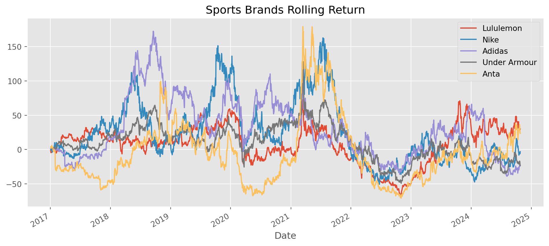
Simulating Stocks Growth
This is a fast way of simulate an stock price accumulative return.
rand_walk = pd.Series(sp.stats.norm.rvs(loc=0.0005, scale=0.012, size=3000))
(1 + rand_walk).cumprod().plot(figsize=(12, 5), grid=True)
plt.show()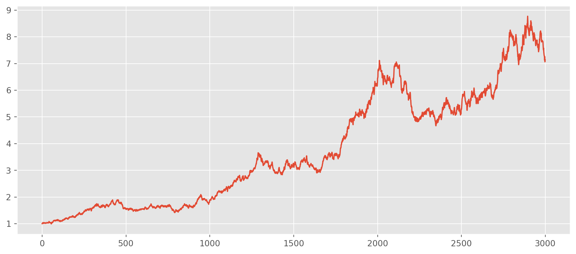
np.random.choice(10, 20)array([4, 6, 7, 0, 2, 8, 8, 3, 6, 7, 7, 3, 3, 3, 1, 2, 0, 7, 8, 3])daily_lulu.values.flatten() is used for turning dataframe into a 1-d array, np.random.choice is for choosing size of len(daily_lulu) observations out of the whole 1-d array with equal weight.
lulu = yf.download(tickers="LULU", start="2010-1-1", end=dt.datetime.today())[
    "Close"
].to_frame()
daily_lulu = lulu.pct_change().dropna()
lulu_simu = pd.Series(np.random.choice(daily_lulu.values.flatten(), len(daily_lulu)))
sns.displot(lulu_simu)
plt.show()
[*********************100%***********************] 1 of 1 completed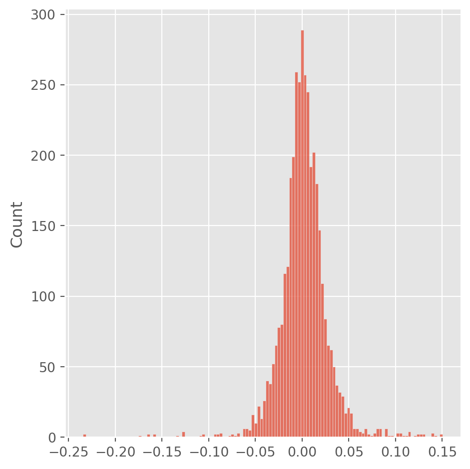
first = lulu["Close"].first("D")
ts_holder = pd.concat([first, 1 + lulu_simu])
ts_holder = ts_holder.cumprod()
ts_holder.index = lulu.index
lulu["lulu_sim_price"] = ts_holder
lulu.plot(figsize=(12, 5), grid=True)
plt.show()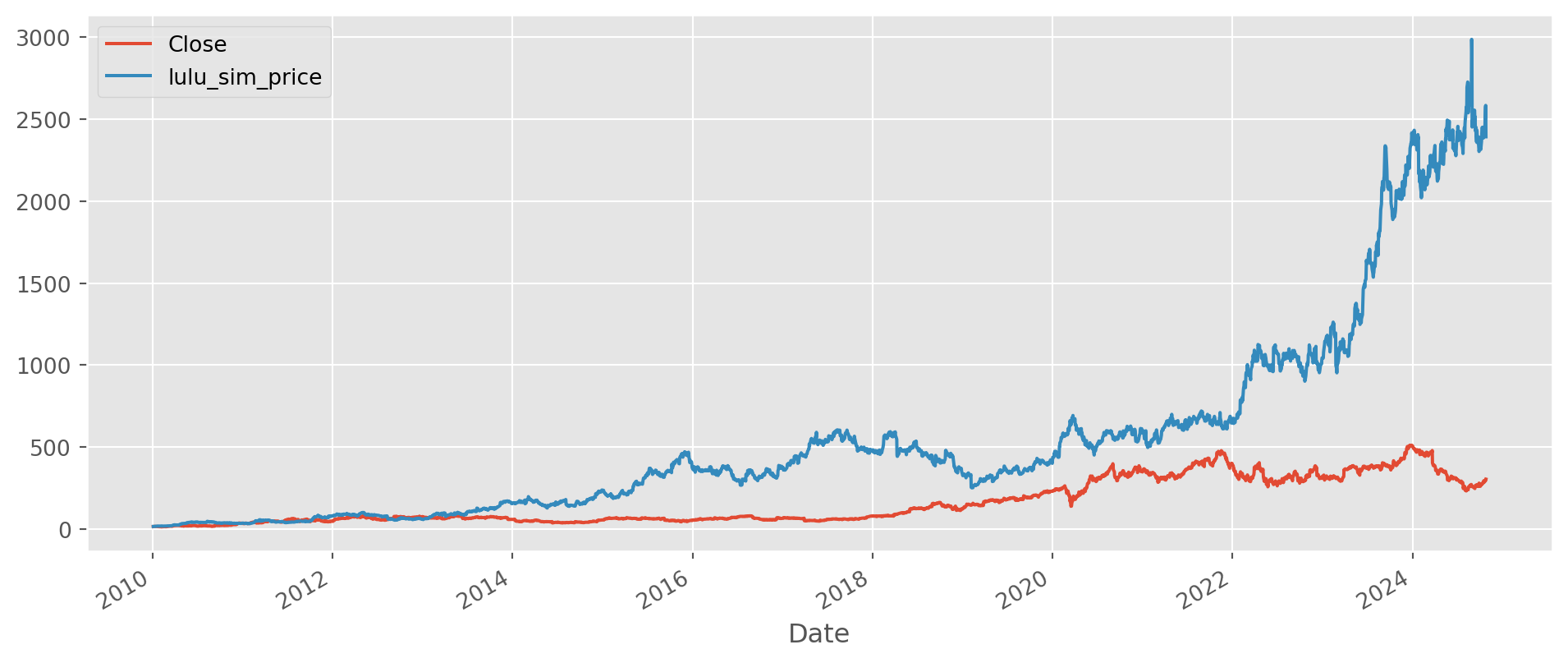
Listings Example
nasdaq = pd.read_csv("../dataset/nasdaq_listings.csv", na_values=True)nasdaq.head()| Stock Symbol | Company Name | Last Sale | Market Capitalization | IPO Year | Sector | Industry | Last Update | |
|---|---|---|---|---|---|---|---|---|
| 0 | AAPL | Apple Inc. | 141.05 | 7.400000e+11 | 1980 | Technology | Computer Manufacturing | 4/26/17 |
| 1 | GOOGL | Alphabet Inc. | 840.18 | 5.810000e+11 | NAN | Technology | Computer Software: Programming, Data Processing | 4/24/17 |
| 2 | GOOG | Alphabet Inc. | 823.56 | 5.690000e+11 | 2004 | Technology | Computer Software: Programming, Data Processing | 4/23/17 |
| 3 | MSFT | Microsoft Corporation | 64.95 | 5.020000e+11 | 1986 | Technology | Computer Software: Prepackaged Software | 4/26/17 |
| 4 | AMZN | Amazon.com, Inc. | 884.67 | 4.220000e+11 | 1997 | Consumer Services | Catalog/Specialty Distribution | 4/24/17 |
nasdaq.set_index("Stock Symbol", inplace=True)nasdaq.dropna(subset=["Sector"], inplace=True) # remove companies without sector infonasdaq["Market Capitalization"] /= 1e6nasdaq.info()<class 'pandas.core.frame.DataFrame'>
Index: 1115 entries, AAPL to FARO
Data columns (total 7 columns):
# Column Non-Null Count Dtype
--- ------ -------------- -----
0 Company Name 1115 non-null object
1 Last Sale 1115 non-null float64
2 Market Capitalization 1115 non-null float64
3 IPO Year 1115 non-null object
4 Sector 1115 non-null object
5 Industry 1115 non-null object
6 Last Update 1115 non-null object
dtypes: float64(2), object(5)
memory usage: 69.7+ KBtop_comp = (
nasdaq.groupby(["Sector"])["Market Capitalization"]
.nlargest(1)
.sort_values(ascending=False)
)
top_compSector Stock Symbol
Technology AAPL 740000.000000
Consumer Services AMZN 422000.000000
Health Care AMGN 119000.000000
Consumer Non-Durables KHC 111000.000000
Miscellaneous PCLN 85496.045967
Public Utilities TMUS 52930.713577
Capital Goods TSLA 49614.832848
NAN QQQ 46376.760000
Transportation CSX 43005.669415
Finance CME 39372.418940
Consumer Durables CPRT 13620.922869
Energy FANG 9468.718827
Basic Industries STLD 7976.835456
Name: Market Capitalization, dtype: float64tickers = top_comp.index.get_level_values(
1
) # use 0, 1...any integer to refer to the level of indices
tickers = tickers.tolist()
tickers['AAPL',
'AMZN',
'AMGN',
'KHC',
'PCLN',
'TMUS',
'TSLA',
'QQQ',
'CSX',
'CME',
'CPRT',
'FANG',
'STLD']columns = ["Company Name", "Market Capitalization", "Last Sale"]
comp_info = nasdaq.loc[tickers, columns].sort_values(
by="Market Capitalization", ascending=False
)
comp_info["no_share"] = comp_info["Market Capitalization"] / comp_info["Last Sale"]
comp_info.dtypesCompany Name object
Market Capitalization float64
Last Sale float64
no_share float64
dtype: objectcomp_info| Company Name | Market Capitalization | Last Sale | no_share | |
|---|---|---|---|---|
| Stock Symbol | ||||
| AAPL | Apple Inc. | 740000.000000 | 141.05 | 5246.366537 |
| AMZN | Amazon.com, Inc. | 422000.000000 | 884.67 | 477.014028 |
| AMGN | Amgen Inc. | 119000.000000 | 161.61 | 736.340573 |
| KHC | The Kraft Heinz Company | 111000.000000 | 91.50 | 1213.114754 |
| PCLN | The Priceline Group Inc. | 85496.045967 | 1738.77 | 49.170417 |
| TMUS | T-Mobile US, Inc. | 52930.713577 | 64.04 | 826.525821 |
| TSLA | Tesla, Inc. | 49614.832848 | 304.00 | 163.206687 |
| QQQ | PowerShares QQQ Trust, Series 1 | 46376.760000 | 130.40 | 355.650000 |
| CSX | CSX Corporation | 43005.669415 | 46.42 | 926.446993 |
| CME | CME Group Inc. | 39372.418940 | 115.87 | 339.798213 |
| CPRT | Copart, Inc. | 13620.922869 | 29.65 | 459.390316 |
| FANG | Diamondback Energy, Inc. | 9468.718827 | 105.04 | 90.143934 |
| STLD | Steel Dynamics, Inc. | 7976.835456 | 32.91 | 242.383332 |
stocks = yf.download(tickers=tickers, start="2000-1-1", end=dt.datetime.today())[
    "Close"
]
[ 0% ][******* 15% ] 2 of 13 completed[*********** 23% ] 3 of 13 completed[*************** 31% ] 4 of 13 completed[****************** 38% ] 5 of 13 completed[**********************46% ] 6 of 13 completed[**********************54%* ] 7 of 13 completed[**********************62%***** ] 8 of 13 completed[**********************69%******** ] 9 of 13 completed[**********************77%************ ] 10 of 13 completed[**********************85%**************** ] 11 of 13 completed[**********************92%******************* ] 12 of 13 completed[*********************100%***********************] 13 of 13 completed
1 Failed download:
['PCLN']: YFPricesMissingError('$%ticker%: possibly delisted; no price data found (1d 2000-1-1 -> 2024-10-27 17:37:40.715625)')stocks.head()| Ticker | AAPL | AMGN | AMZN | CME | CPRT | CSX | FANG | KHC | PCLN | QQQ | STLD | TMUS | TSLA |
|---|---|---|---|---|---|---|---|---|---|---|---|---|---|
| Date | |||||||||||||
| 2000-01-03 00:00:00+00:00 | 0.999442 | 62.9375 | 4.468750 | NaN | 0.812500 | 1.718750 | NaN | NaN | NaN | 94.75000 | 3.984375 | NaN | NaN |
| 2000-01-04 00:00:00+00:00 | 0.915179 | 58.1250 | 4.096875 | NaN | 0.710938 | 1.666667 | NaN | NaN | NaN | 88.25000 | 3.765625 | NaN | NaN |
| 2000-01-05 00:00:00+00:00 | 0.928571 | 60.1250 | 3.487500 | NaN | 0.705729 | 1.701389 | NaN | NaN | NaN | 86.00000 | 4.046875 | NaN | NaN |
| 2000-01-06 00:00:00+00:00 | 0.848214 | 61.1250 | 3.278125 | NaN | 0.656250 | 1.777778 | NaN | NaN | NaN | 80.09375 | 4.093750 | NaN | NaN |
| 2000-01-07 00:00:00+00:00 | 0.888393 | 68.0000 | 3.478125 | NaN | 0.731771 | 1.777778 | NaN | NaN | NaN | 90.00000 | 4.234375 | NaN | NaN |
returns = (stocks.iloc[-1] / stocks.loc["2018-1-2"] - 1) * 100
returns.plot(kind="barh", figsize=(12, 6), grid=True)
plt.show()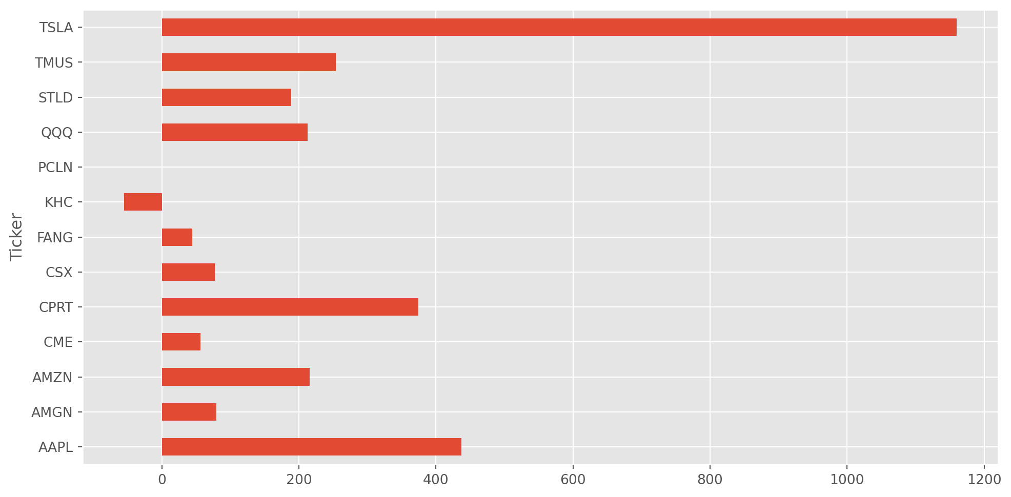
Group By Month
Grouping by month is just for demonstrative purpose, not really meaningful operation in my opinion.
stock_index = pdr.data.DataReader(
    name=["SP500", "NIKKEI225", "NASDAQCOM"],
    data_source="fred",
    start="2001-1-1",
    end=dt.datetime.today(),
)
stock_index.groupby(stock_index.index.month).mean().plot(
subplots=True, figsize=(15, 10)
)
plt.show()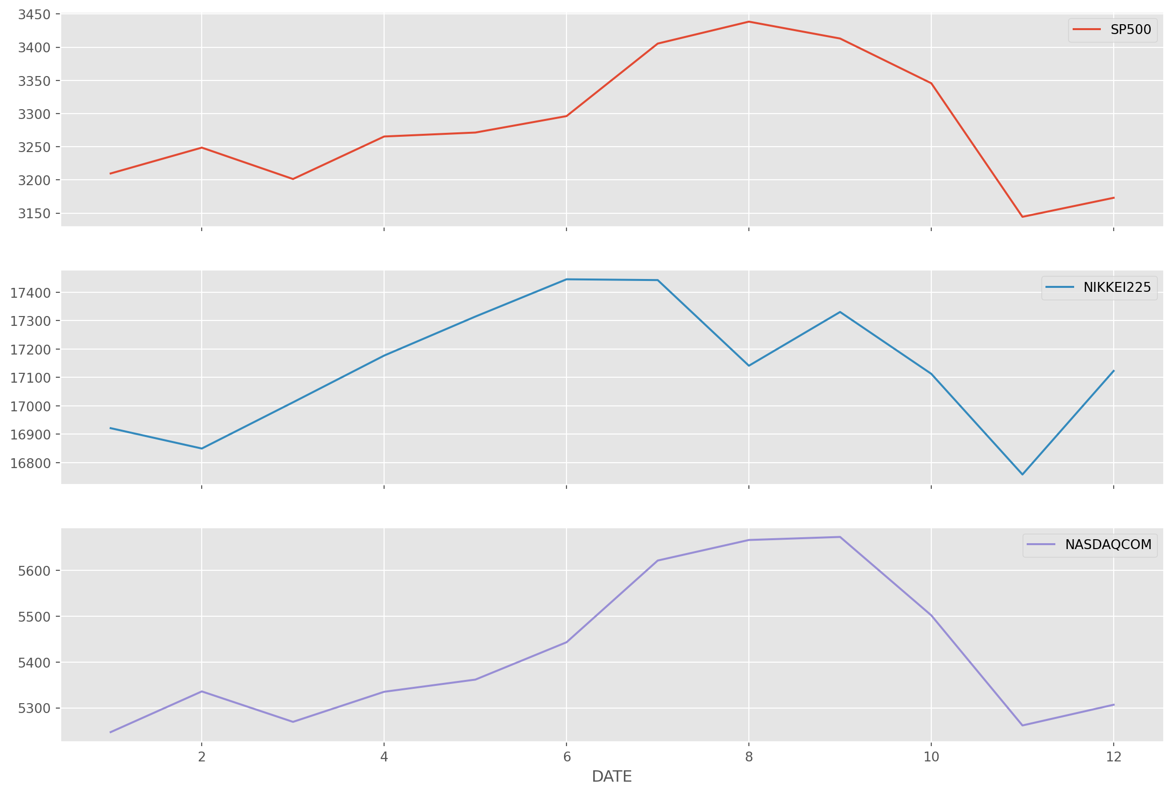
stock_index.groupby(stock_index.index.day).mean().plot(subplots=True, figsize=(15, 10))
plt.show()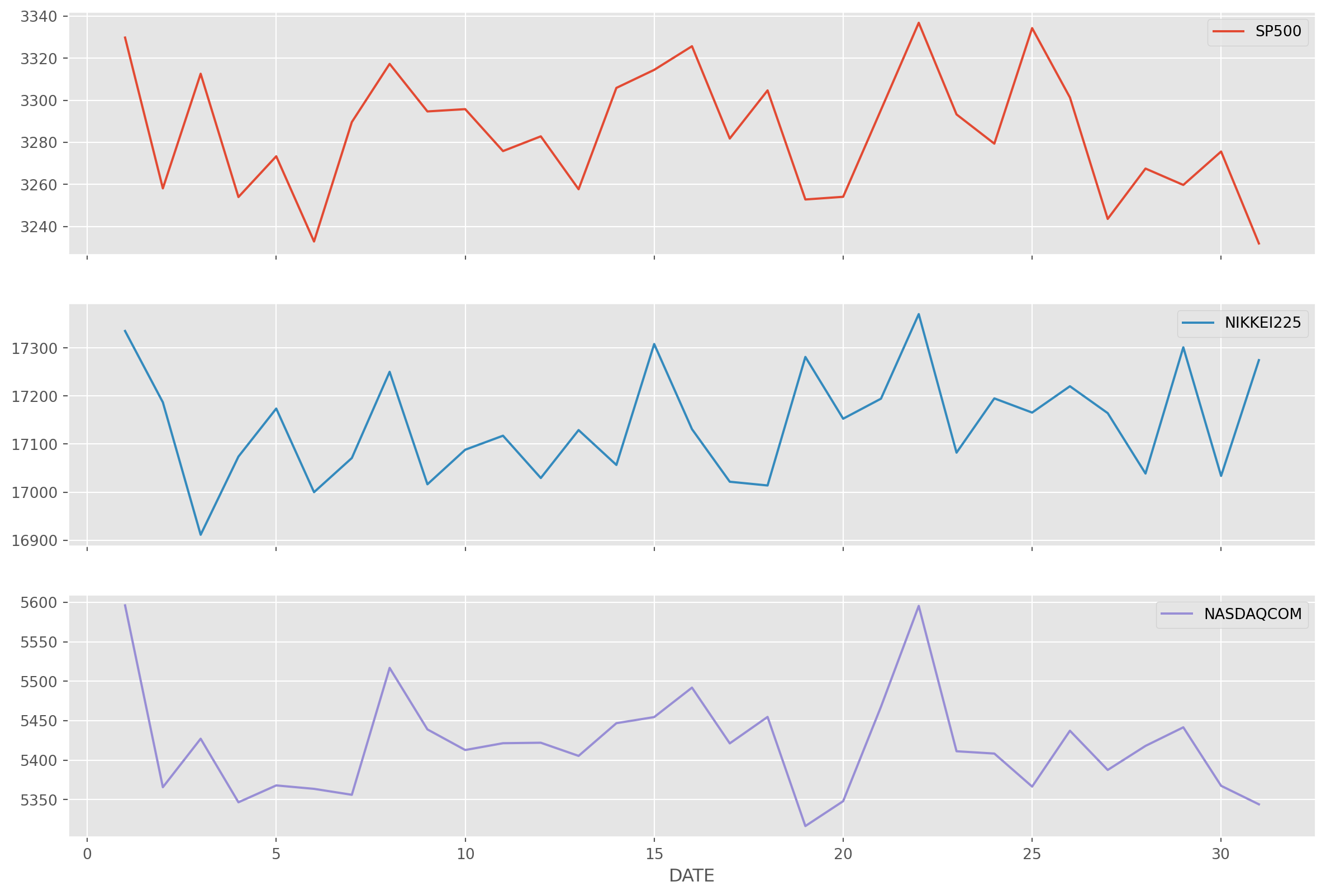
Boxplot
stock_index[["SP500"]].diff().boxplot()
plt.show()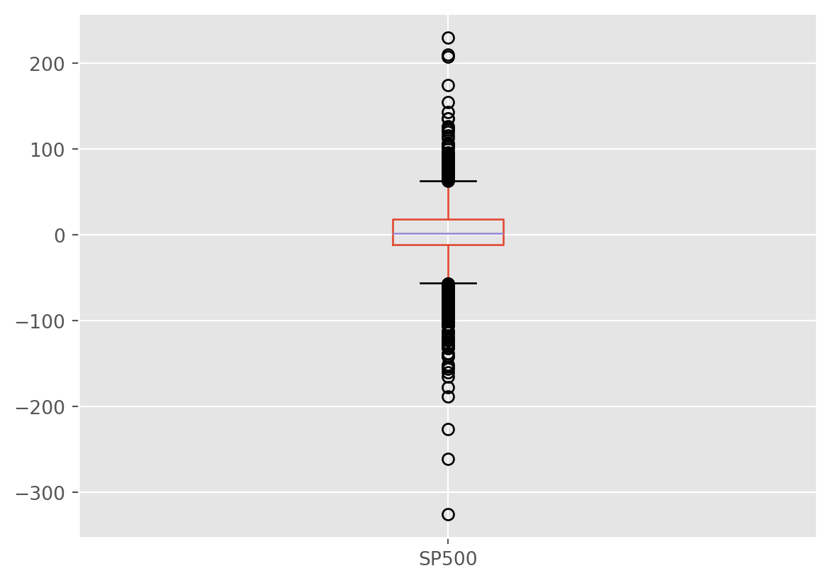
stock_index[["SP500"]].plot(kind="hist", bins=100)
plt.show()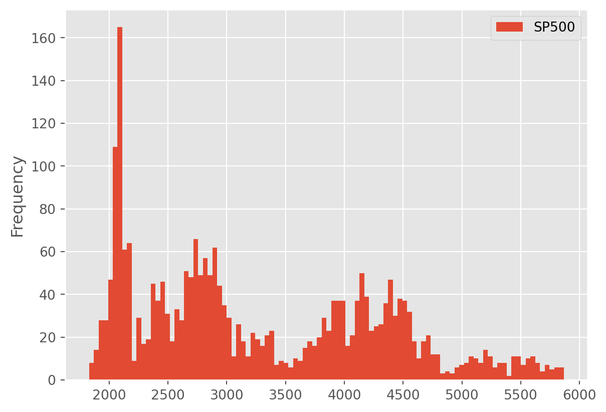
stock_index[["SP500"]].plot(kind="density")
plt.show()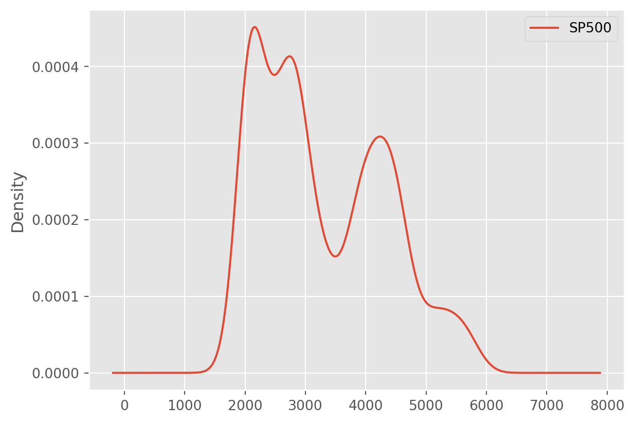
Plotting Autocorrelation
fig = tsaplots.plot_acf(stock_index["SP500"].dropna())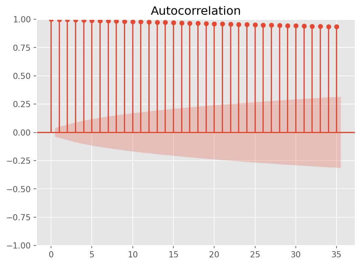
fig = tsaplots.plot_pacf(stock_index["SP500"].dropna())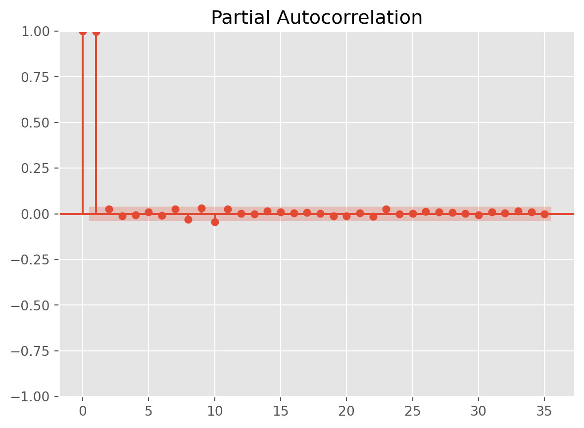
Decomposition
A common view to an economic time series is that it can be decomposed into three elements: trend, seasonality and cycles.
tot_constr_China = pdr.data.DataReader(
    name=["CHNPRCNTO01MLQ"],
    data_source="fred",
    start="2001-1-1",
    end=dt.datetime.today(),
)
tot_constr_China.columns = ["constru_data"]
statsmodels has a naive decomposition function, it could be used for a fast statistical inspection, but not recommended.
decomp = sm.tsa.seasonal_decompose(tot_constr_China["constru_data"])The top plot shows the original data.
plt.rcParams["figure.figsize"] = 16, 10
fig = decomp.plot()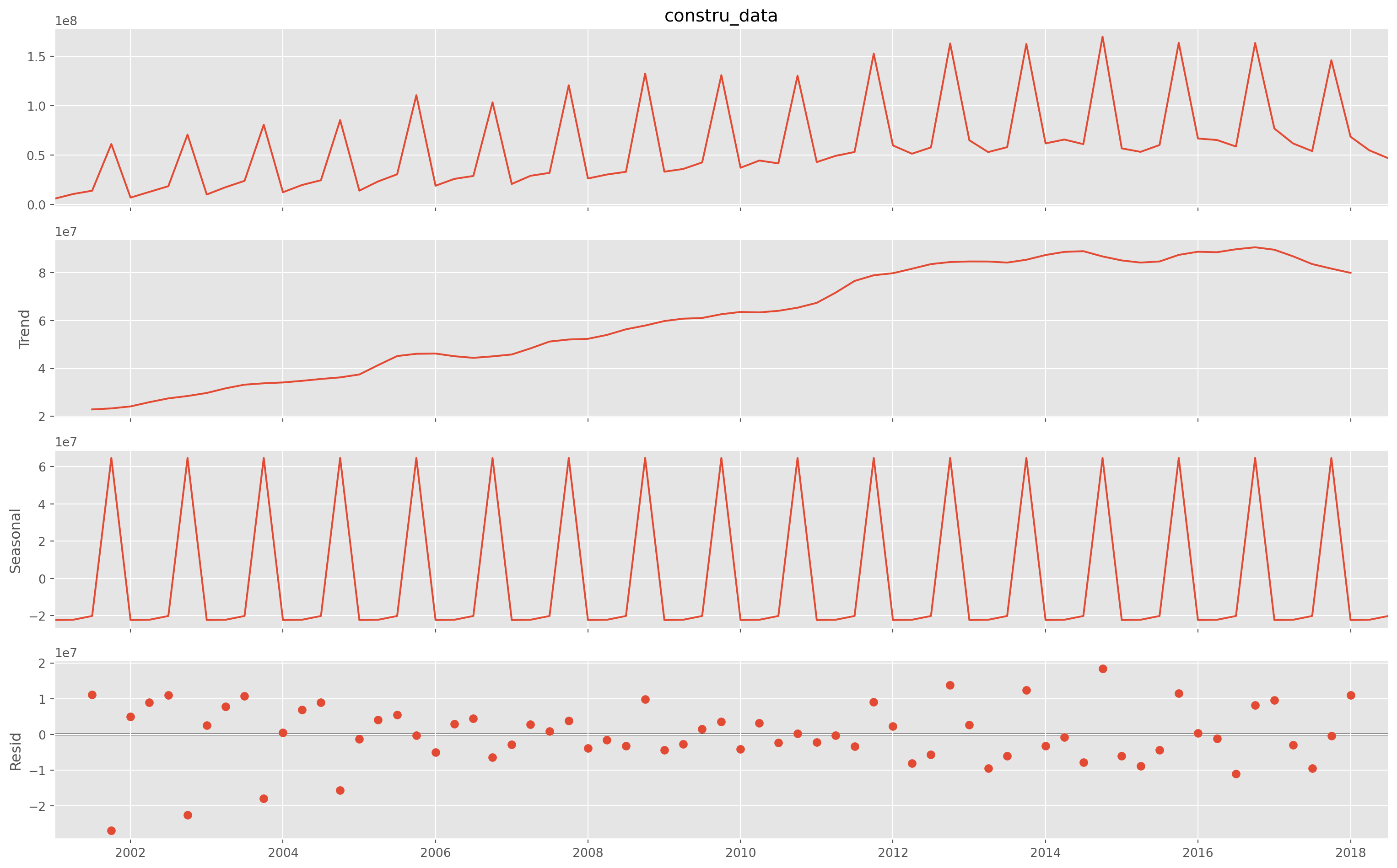
Area Plot
Area plot are each to read.
df = pdr.data.DataReader(
    name=["PCE", "W068RCQ027SBEA", "BOPGSTB"],
    data_source="fred",
    start="2001-1-1",
    end=dt.datetime.today(),
)
df.columns = ["PCE", "Gov_Exp", "Trade_Ba"]
df["Trade_Ba"] = df["Trade_Ba"] / 1000  # convert to billion unit
df["Gov_Exp"] = df["Gov_Exp"].interpolate()df.plot.area(stacked=False)
plt.show()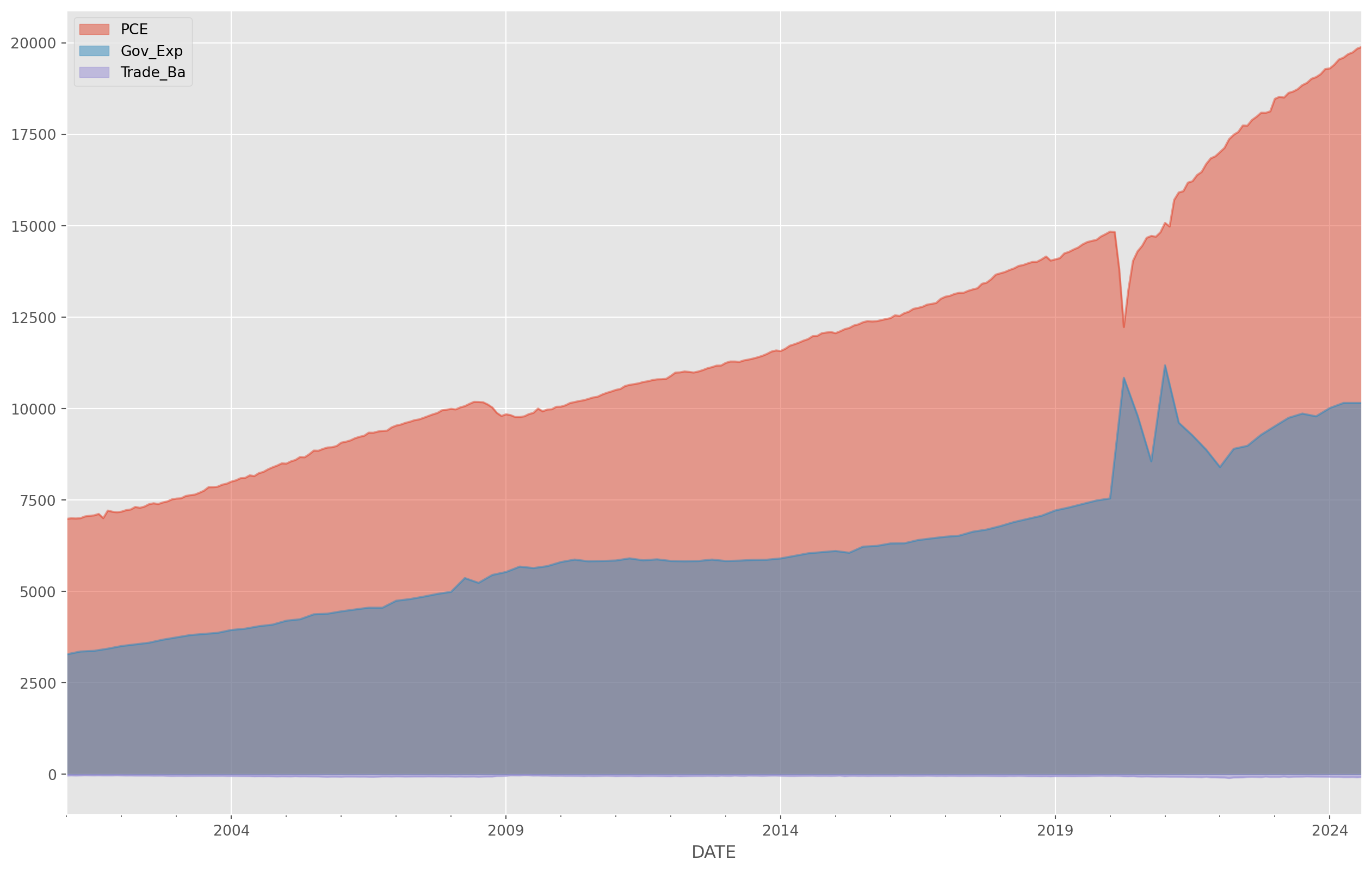
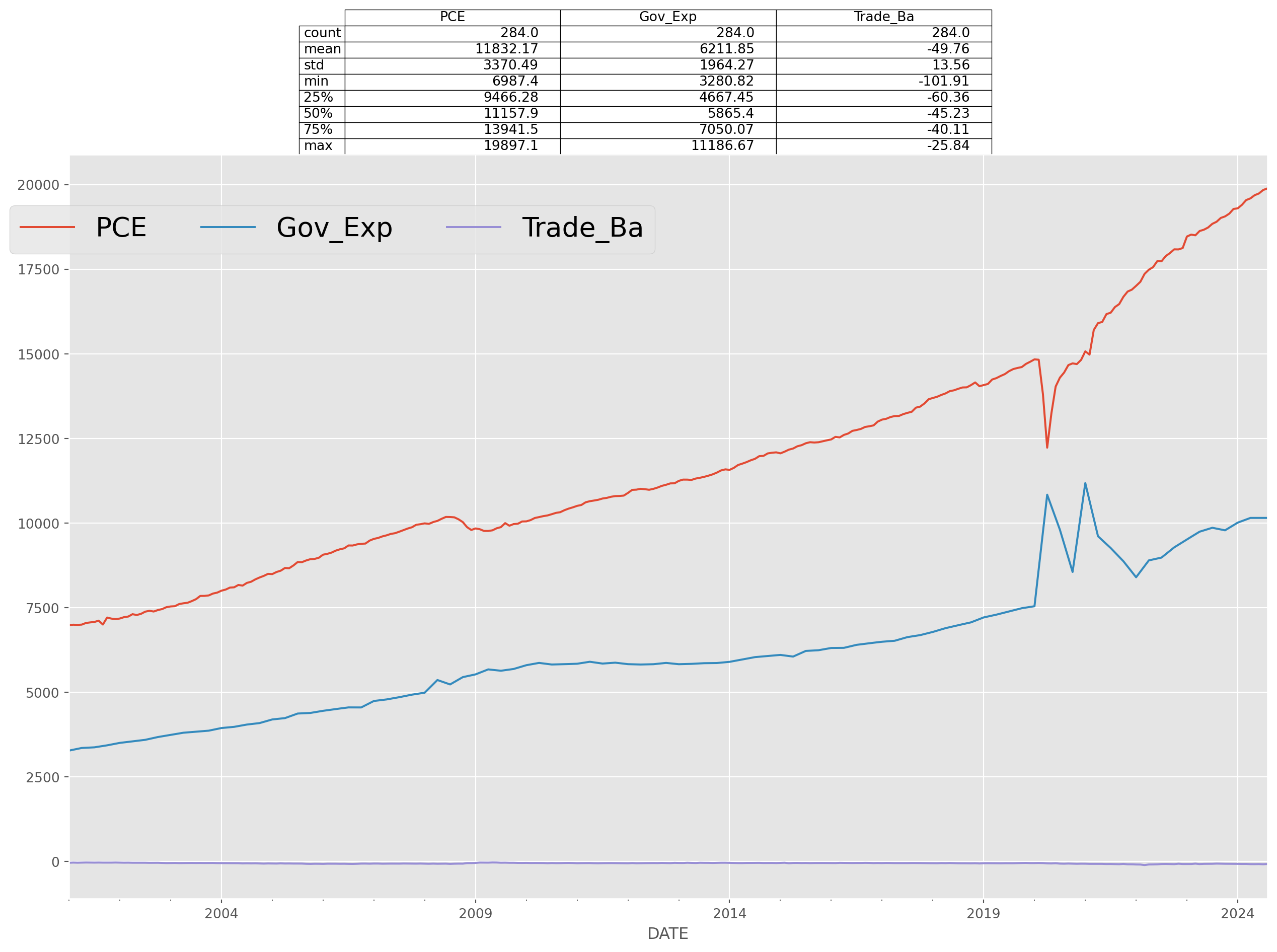
Adding Summary Statistics
ax = df.plot()
df_summary = df.describe()

ax.table(
    cellText=np.round(df_summary.values, 2),
    colWidths=[0.18] * len(df_summary.columns),
    rowLabels=df_summary.index,
    colLabels=df_summary.columns,
    loc="top",
)
ax.legend(loc="best", bbox_to_anchor=(0.5, 0.95), ncol=3, fontsize=20)
plt.show()